In single-variable calculus, we studied functions of the form \(y=f(x)\text{,}\) which result in graphs that are curves in the \(xy\)-plane. In linear algebra or the previous chapter, we studied vectors, which represent magnitude and direction but are static.
In this section, we combine these concepts to define vector-valued functions. By allowing the components of a vector to be functions of a parameter \(t\) (often representing time), we can describe dynamic motion in space.
Imagine you are tracking the position of a particle moving in \(\R^2\text{.}\) At any time \(t\text{,}\) the position of the particle can be represented by a vector \(\v{r}(t) = \la x(t), y(t) \ra\text{,}\) where \(x(t)\) and \(y(t)\) are functions that describe the particle’s coordinates in the plane. As time progresses, the tip of the vector \(\v{r}(t)\) traces out a path in the plane, known as a Plane Curve.
Similarly, if the particle is moving in \(\R^3\text{,}\) at any time \(t\text{,}\) the position of the particle can be represented by a vector \(\v{r}(t) = \la x(t), y(t), z(t) \ra\text{,}\) where \(x(t)\text{,}\)\(y(t)\text{,}\) and \(z(t)\) are functions that describe the particle’s coordinates in \(\R^3\text{.}\) As time progresses, the tip of the vector \(\v{r}(t)\) traces out a path in space, known as a Space Curve.
The function \(\v{r}(t)\) is called a Vector-Valued Function because it assigns a vector to each value of the parameter \(t\text{.}\) In \(\R^3\text{,}\) a vector-valued function is typically expressed as
where \(t\) is called the parameter of the function, and \(x(t)\text{,}\)\(y(t)\text{,}\) and \(z(t)\) are the component or coordinate functions that determine the coordinates of the vector in space.
Now that we have a function, we want to understand its domain. The domain of a vector-valued function is the set of all possible values of the parameter \(t\) for which all the component functions are defined.
The domain of \(\v{r}(t)\) must be the set of all \(t\) values for which all three component functions are defined. How can we find a set of \(t\) values that works for all three component functions?
To find the domain of \(\v{r}(t)\text{,}\) we need to find the intersection of the domains of the three component functions to ensure that all components are defined. That is, the domain of \(\v{r}(t)\) is
There are two things we are discussing here: the path parametrized by \(\v{r}(t)\) and the curve \(\c{C}\) traced by the tip of the vector \(\v{r}(t)\text{.}\)
The path is the vector-valued function \(\v{r}(t)\) itself. It describes how the curve is traversed as the parameter \(t\) varies. You can think of it as the specific trip you take along that road.
The curve \(\c{C}\) is the set of points in space. It is a static geometric object left behind by the path. You can think of it as the physical road on a map.
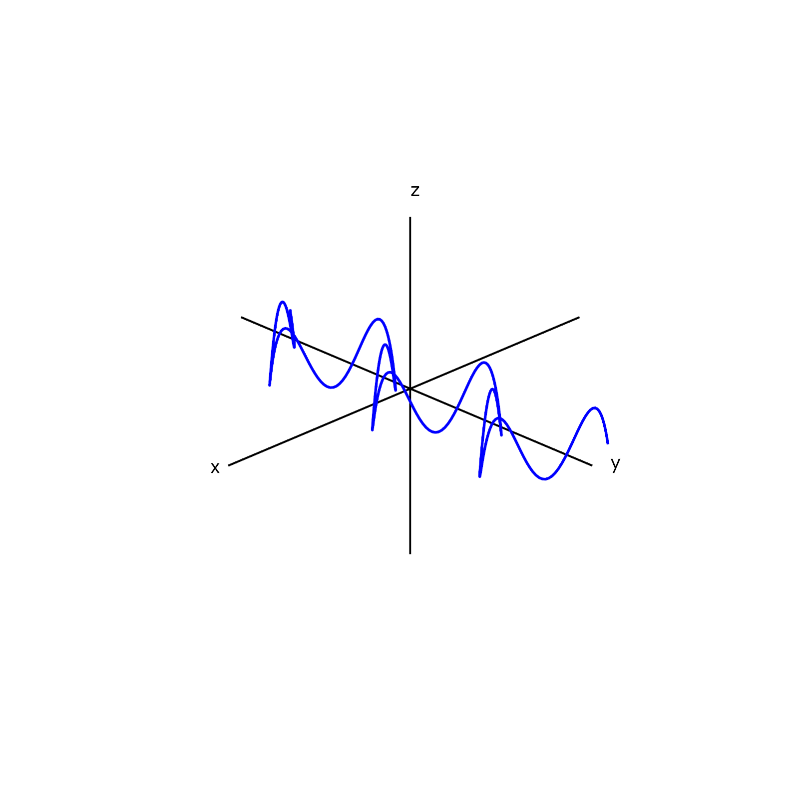
The path is the function \(\v{r}(t)\) itself, which describes how the curve is traced out as \(t\) varies from \(-3\pi\) to \(3\pi\) (see the figure below).
The curve \(\c{C}\) is the set of points in space traced out by the tip of the vector \(\v{r}(t)\) as \(t\) varies from \(-3\pi\) to \(3\pi\) (see the figure below).
Next, let’s discuss how to describe the curve traced by a vector-valued function. One way to do so is to eliminate one variable through projection onto a coordinate plane. Then we can easily describe the resulting curve in two dimensions.
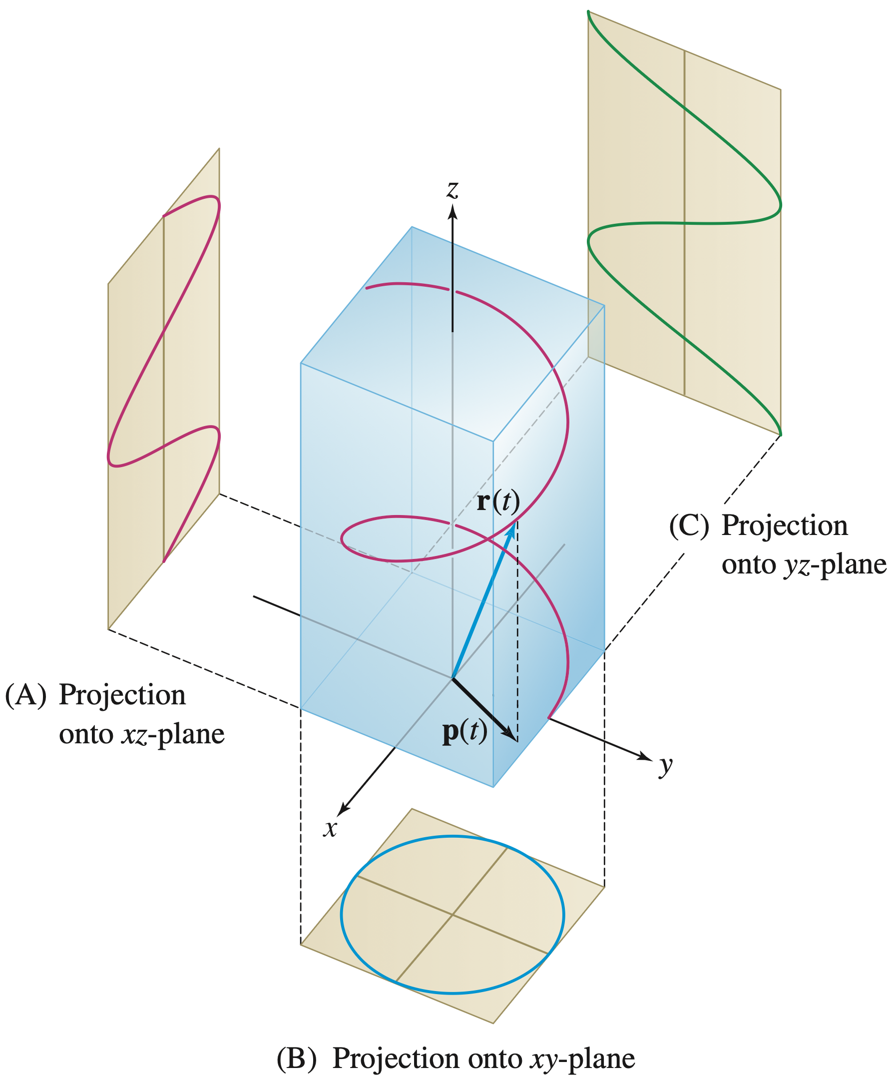
The curve traced by \(\v{r}(t) = \la -\sin(t), \cos(t), t \ra\) for \(t \geq 0\) is called a helix. Describe the curve in terms of its projections onto the coordinate planes.
We can project the curve onto the standard \(xy\)-plane, \(yz\)-plane, and \(xz\)-plane by setting the appropriate coordinate to zero. Then we can observe the resulting curves in two dimensions.
By setting \(z = 0\text{,}\) we project the curve onto the \(xy\)-plane. The projection is given by \(\v{p}(t) = \la -\sin(t),\cos(t),0 \ra\text{.}\) This implies that
By setting \(x = 0\text{,}\) we project the curve onto the \(yz\)-plane. The projection is given by \(\la 0, \cos(t), t \ra\text{.}\) This implies that
We can simply express \(y\) in terms of \(z\) as \(y = \cos(z)\text{.}\) Hence, the projection onto the \(yz\)-plane is a cosine curve that oscillates between \(1\) and \(-1\) as \(z\) increases.
By setting \(y = 0\text{,}\) we project the curve onto the \(xz\)-plane. The projection is given by \(\la -\sin(t), 0, t \ra\text{.}\) This implies that
We can simply express \(x\) in terms of \(z\) as \(x = -\sin(z)\text{.}\) Hence, the projection onto the \(xz\)-plane is a negative sine curve that oscillates between \(1\) and \(-1\) as \(z\) increases.
Projections are useful not only for visualizing curves in \(\R^3\text{,}\) but also for analyzing the curves in \(\R^3\text{.}\) That is, by studying the projections onto the coordinate planes, we can obtain the vector-valued function of the curve in \(\R^3\text{.}\)
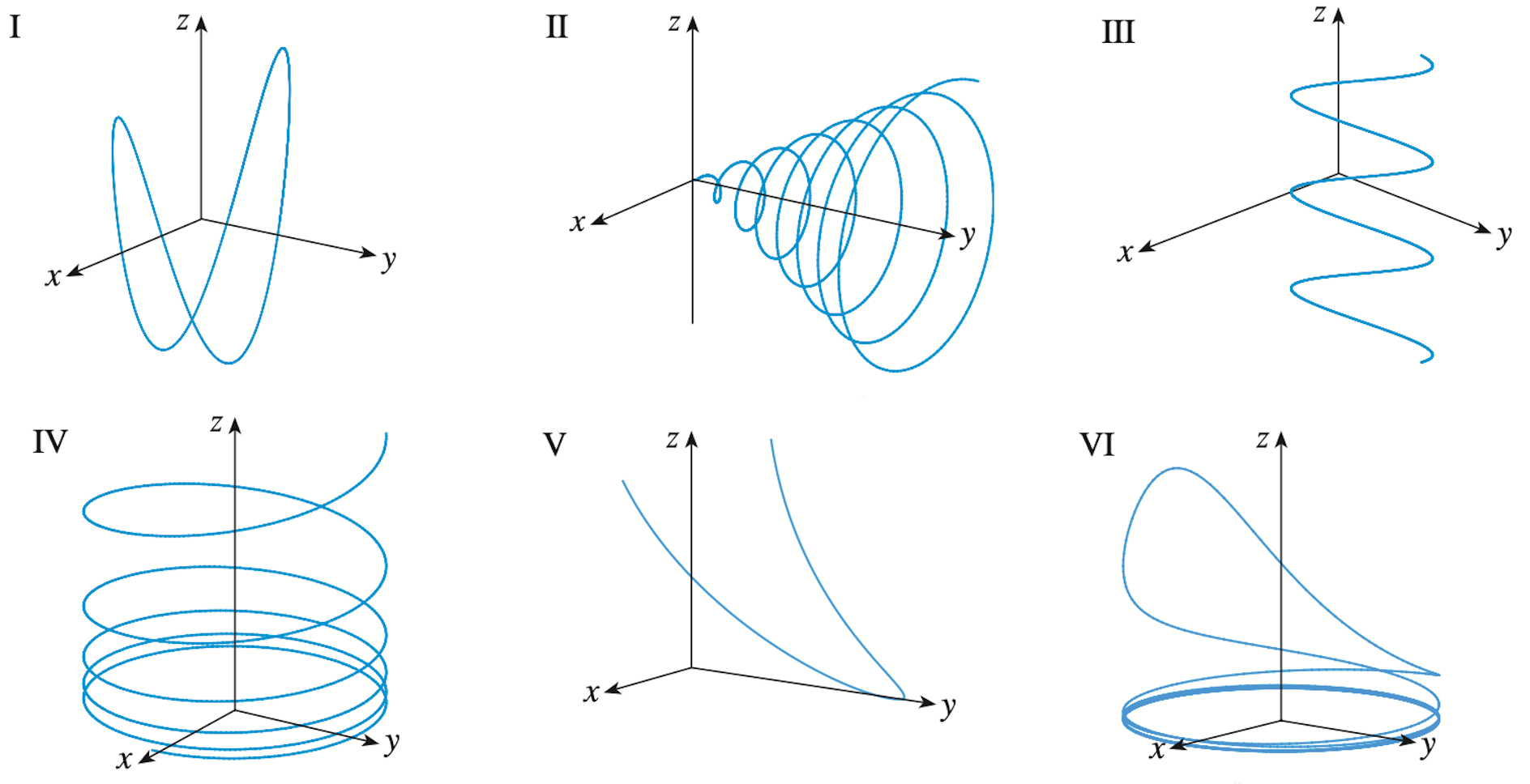
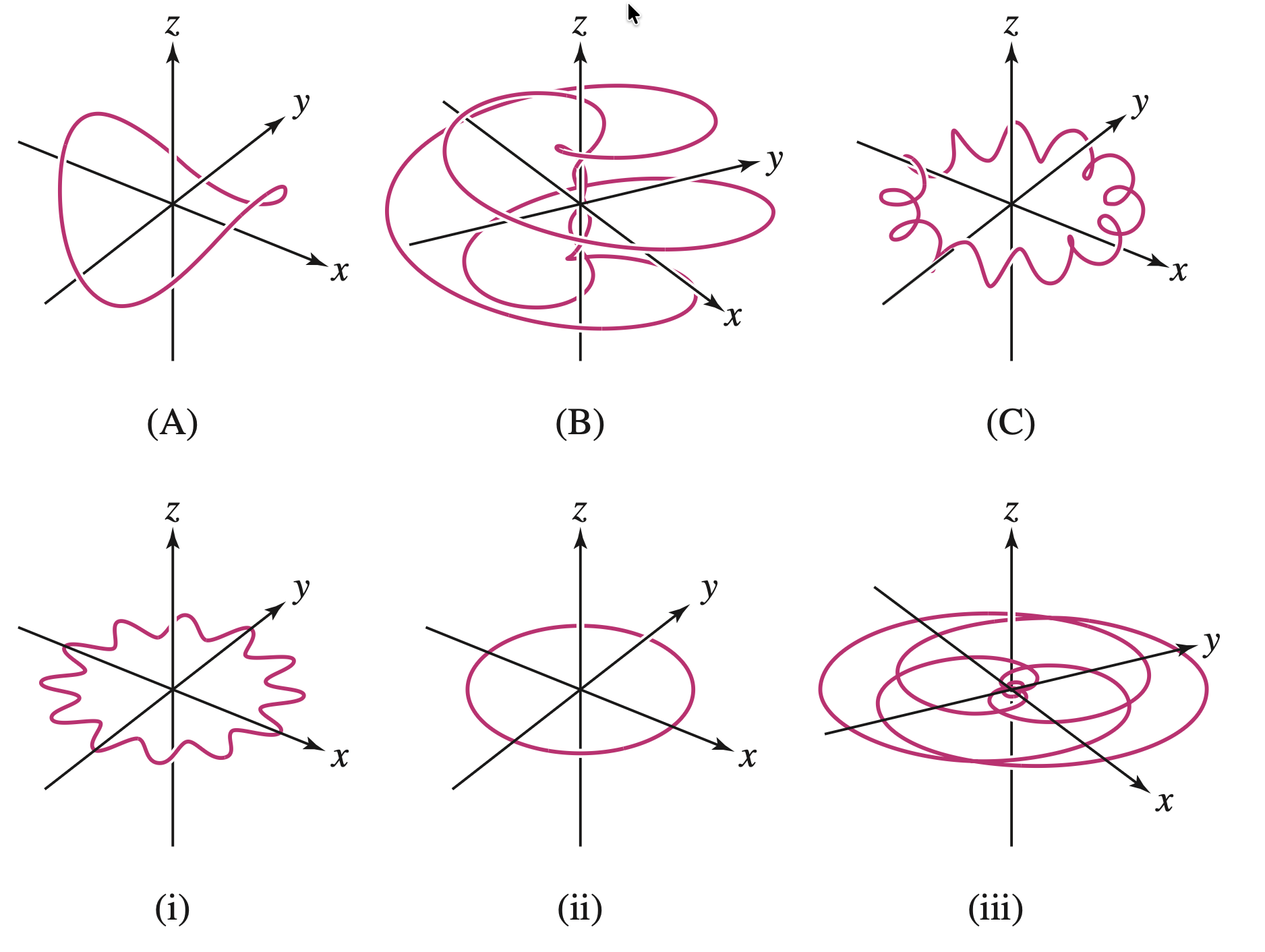
To match the vector-valued functions with the space curves, we can analyze the projections of each curve onto the coordinate planes. By examining the behavior of the projections, we can identify which vector-valued function corresponds to each curve.
\(\mathbf{r}(t) = \langle t \cos(t), t, t \sin(t) \rangle\) corresponds to graph II. Observe that \(x^2 + z^2 = t^2 \cos^2(t) + t^2 \sin^2(t) = t^2 = y^2\text{.}\) This indicates the curve lies on the cone \(y^2 = x^2 + z^2\text{.}\) The spiral radius increases as the variable \(y\) increases, which matches graph II.
\(\mathbf{r}(t) = \langle \cos(t), \sin(t), \frac{1}{1+t^2} \rangle\) corresponds to graph VI. Here, \(x^2 + y^2 = 1\text{,}\) so the curve lies on a cylinder. The \(z\)-component \(z = \frac{1}{1+t^2}\) peaks at \(z=1\) and approaches \(0\) as \(t \to \pm \infty\text{.}\) Graph VI shows a spiral on a cylinder that rises to a peak and flattens out towards the bottom, matching this behavior.
\(\mathbf{r}(t) = \langle t, \frac{1}{1+t^2}, t^2 \rangle\) corresponds to graph V. Notice that \(z = t^2 = x^2\text{,}\) meaning the curve lies on the parabolic cylinder \(z = x^2\text{.}\) As \(x\) moves away from zero, \(z\) increases quadratically while \(y\) approaches zero. This matches the parabolic track seen in graph V.
\(\mathbf{r}(t) = \langle \cos(t), \sin(t), \cos(2t) \rangle\) corresponds to graph I. The curve lies on the cylinder \(x^2 + y^2 = 1\text{.}\) Since all components are periodic, the curve is a closed loop. The \(z\)-component oscillates between \(-1\) and \(1\) with a frequency double that of the rotation in \(xy\text{,}\) creating the "saddle" shape seen in graph I.
\(\mathbf{r}(t) = \langle \cos(8t), \sin(8t), e^{0.8t} \rangle\) corresponds to graph IV. This describes a helix on the cylinder \(x^2 + y^2 = 1\text{.}\) The \(z\)-component grows exponentially, which means the vertical spacing (pitch) between the coils increases as the curve rises. This is clearly visible in graph IV.
\(\mathbf{r}(t) = \langle \cos^2(t), \sin^2(t), t \rangle\) corresponds to graph III. Observe that \(x + y = \cos^2(t) + \sin^2(t) = 1\text{.}\) The curve is confined to the plane \(x + y = 1\text{.}\) As \(z=t\) increases, the point oscillates along a line segment in the \(xy\)-plane, creating the wave-like shape on a flat plane seen in graph III.
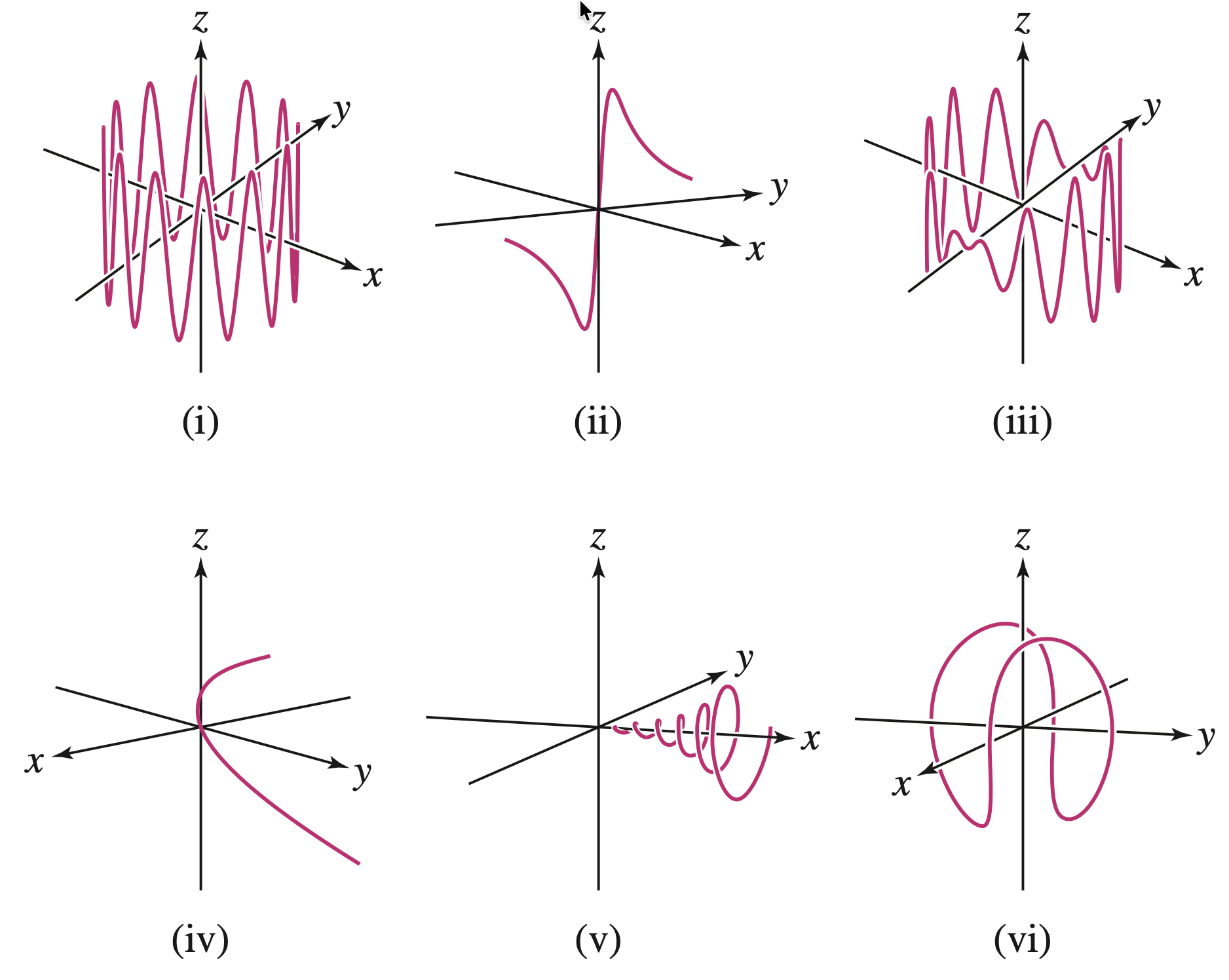
Graph I matches equation (d) \(\mathbf{r}(t) = \langle \cos(t), \sin(t), \cos(2t) \rangle\text{.}\) This is the only closed loop among the graphs. Mathematically, this corresponds to the only function where all three components are periodic, meaning the curve eventually retraces its path.
Graph II matches equation (a) \(\mathbf{r}(t) = \langle t \cos(t), t, t \sin(t) \rangle\text{.}\) The graph shows a spiral expanding along the \(y\)-axis, forming a cone. This matches equation (a) because the radius of the spiral in the \(xz\)-plane is \(\sqrt{(t\cos t)^2 + (t\sin t)^2} = |t|\text{,}\) which equals the distance along the \(y\)-axis (\(|y|\)).
Graph III matches equation (f) \(\mathbf{r}(t) = \langle \cos^2(t), \sin^2(t), t \rangle\text{.}\) The graph shows a wave confined to a flat vertical plane. This matches equation (f) because \(x + y = \cos^2(t) + \sin^2(t) = 1\text{,}\) meaning the curve lies entirely on the plane \(x + y = 1\text{.}\)
Graph IV matches equation (e) \(\mathbf{r}(t) = \langle \cos(8t), \sin(8t), e^{0.8t} \rangle\text{.}\) The graph is a helix where the vertical distance between coils increases (the pitch widens). This matches equation (e) because the \(z\)-component grows exponentially (\(e^{0.8t}\)), causing the curve to rise faster and faster.
Graph V matches equation (c) \(\mathbf{r}(t) = \langle t, \frac{1}{1+t^2}, t^2 \rangle\text{.}\) The graph shows a parabolic shape where the \(y\)-coordinate approaches zero as the curve rises. This matches equation (c) because \(z = x^2\) (a parabola) and \(y = \frac{1}{1+t^2}\text{,}\) which approaches 0 as \(t \to \infty\text{.}\)
Graph VI matches equation (b) \(\mathbf{r}(t) = \langle \cos(t), \sin(t), \frac{1}{1+t^2} \rangle\text{.}\) The graph depicts a spiral that is confined near the \(z=0\) plane, rising to a peak and falling back. This corresponds to the "bell curve" behavior of the \(z\)-component \(\frac{1}{1+t^2}\text{,}\) which is bounded between 0 and 1.
SubsectionParametrization of Vector-Valued Functions
Parametrization is the process of expressing a curve using a vector-valued function. That is, given a curve in space, we want to find a vector-valued function \(\v{r}(t)\) that traces out the curve as \(t\) varies over some interval.
From the first surface, we have \(x^2 + y^2 = 1\text{,}\) so \(x = \pm\sqrt{1-y^2}\text{,}\) where \(-1 \leq y \leq 1\text{.}\) From the second surface, we have \(z = 2 - y\text{.}\)
Note: the \(\pm\) sign makes the \(x\)-component not a function of \(t\text{.}\) In practice, we would split the parametrization into two separate parts: one for \(x = \sqrt{1-t^2}\) and another for \(x = -\sqrt{1-t^2}\text{,}\) each defined over the interval \(-1 \leq t \leq 1\text{.}\)
Observe that there are infinitely many ways to parametrize a curve. One way to check your answer is to literally graph the curve and the parametrization to see if they match.
We can graph the curves using the GeoGebra 3D Graphing Calculator or other 3D graphing software. If you type "Curve(cos(t),sin(t),2-sin(t),t,0,2 π)" into GeoGebra, you will see that the curve of intersection is a slanted ellipse. If you type "Curve(\sqrt{1-t^2},t,2-t,t,-1,1)" and "Curve(-\sqrt{1-t^2},t,2-t,t,-1,1)", you will also get the same slanted ellipse.
While the ideas in this section doesn’t seem too difficult, it does require some practice to get comfortable with them. For example, Richard knew how to parametrize things because he knows the standard parametrizations of circles and stuff. Practice will help you internalize these concepts!
The problems listed below are assigned to be included in your problem set portfolio. Note that a specific selection of these problems will also form the written homework assignments. I recommend working through all of them to ensure a solid grasp of the material. Reach out to Richard for help if you get stuck or have any questions.
The solutions will be posted after the written homework due dates. If you have any questions about your work, talk to Richard and he is happy to discuss the process with you.
Determine whether the space curve given by \(\v{r}(t) = \la \sin(t), \dfrac{\cos(t)}{2}, t \ra\) intersects the \(z\)-axis, and if it does, determine where.
The curve intersects the \(z\)-axis if there is some value of \(t\) such that both the \(x\) and \(y\)-coordinates of \(\v{r}(t)\) are zero. That is, such that \(\sin(t) = \cos\lp\frac{t}{2}\rp = 0\text{.}\) Now, \(\sin(x) = 0\) when \(x = n\pi\text{,}\) while \(\cos(x) = 0\) when \(x = \frac{\pi}{2} + n\pi = \frac{2n+1}{2}\pi\text{,}\) where \(n\) is an integer. So if \(t = k\pi\text{,}\) then \(\sin(t) = 0\text{,}\) and if, further, \(k = 2n + 1\) is odd, then \(\cos\lp\frac{k}{2}\pi\rp = 0\text{.}\) So this curve intersects the \(z\)-axis whenever \(k\) is an odd integer multiple of \(\pi\text{,}\) at the points \(\lp 0,0,(2n + 1)\pi \rp\text{.}\)
\(y = 0\) is the equation of the \(xz\)-plane. We conclude that. the function traces the circle of radius \(1\text{,}\) centered at th epoint \((0,0,4)\text{,}\) and contained in the \(xz\)-plane.
As the height \(z = t\) increases linearly with time, the \(x\) and \(y\) coordinates trace out points on the circles of increasing radius. We obtain the following curve.
We solve for \(z\) and \(x\) in terms of \(y\text{.}\) From the equation \(y^2 + z^2 = 9\text{,}\) we have \(z^2 = 9 - y^2\text{,}\) so \(z = \pm \sqrt{9 - y^2}\text{.}\) From the second equation, we have
Use sine and cosine to parametrize the intersection of the cylinder \(x^2 + y^2 = 1\) and the plane \(x + y + z = 1\text{.}\) Then describe the projections of this curve onto the three coordinate planes.
To parametrize the intersection, we start with the cylinder equation \(x^2 + y^2 = 1\text{.}\) This suggests using polar coordinates for \(x\) and \(y\text{.}\) Let \(x = \cos(t)\) and \(y = \sin(t)\) for \(0 \leq t \leq 2\pi\text{.}\)
We eliminate \(y\) using the plane equation \(y = 1 - x - z\) and substitute it into the cylinder equation. The projection is the ellipse given by \(x^2 + (1 - x - z)^2 = 1\text{.}\)
We eliminate \(x\) using the plane equation \(x = 1 - y - z\) and substitute it into the cylinder equation. The projection is the ellipse given by \((1 - y - z)^2 + y^2 = 1\text{.}\)
Two paths \(\v{r}_1(t)\) and \(\v{r}_2(t)\) intersect if there is a point \(P\) lying on both curves. We say that \(\v{r}_1(t)\) and \(\v{r}_2(t)\) collide if \(\v{r}_1(t_0) = \v{r}_2(t_0)\) at some point \(t_0\text{.}\)
For the \(y\)-components to match, we must have \(t=3\text{.}\) However, testing \(t=3\) in the \(x\)-equation gives \((3)^3 - 4(3) + 3 = 27 - 12 + 3 = 18 \neq 0\text{.}\) Since no single value of \(t\) satisfies all equations, the particles do not collide.
Simplifying this yields \(t^3 + 6t^2 - 19t - 24 = 0\text{.}\) We check the integer roots of this polynomial (\(t = -1, 3, -8\)) to see if they satisfy our condition from equation (1), \(t^3 - 2t - 3 = 0\text{.}\)
The circle is parallel to the \(yz\)-plane and centered at \((1,2,5)\text{,}\) hence the \(x\)-coordinates of the points on the circle are \(x = 1\text{.}\) The projection of the circle on the \(yz\)-plane is a circle of radius \(2\) centered at \((2,5)\text{.}\) This circle is parametrized by
\begin{equation*}
y = 2 + 2\cos(t) \qquad \text{ and } \qquad z = 5 + 2\sin(t)
\end{equation*}
We conclude that the points on the required circle can be written as \(\lp 1, 2 + 2\cos(t), 5 + 2\sin(t) \rp\text{.}\) This gives the following parametrization
This circle in the horizontal plane \(y = \frac{1}{2}\) has the parametrization
\begin{equation*}
x = \frac{\sqrt{3}}{2} \cos(t) \qquad \text{ and } \qquad z = \frac{\sqrt{3}}{2} \sin(t)
\end{equation*}
Therefore, the points on the intersection of the plane \(y = \frac{1}{2}\) and the sphere \(x^2 + y^2 + z^2 = 1\) can be written in the form \(\lp \frac{\sqrt{3}}{2}\cos(t), \frac{1}{2}, \frac{\sqrt{3}}{2}\sin(t) \rp\text{,}\) yielding the following parametrization