
Section 15.2 Double Integrals over More General Regions

In this section, we expand our toolkit to handle these general regions. The key shift is that at least one set of our integration limits will now be functions rather than numbers. We will learn to classify regions as either vertically simple or horizontally simple.
Mastering this section requires a bit of "geometric detective work." You will need to sketch the region, find intersection points, and decide which variable should be integrated first to make the calculus as smooth as possible. We will also see how double integrals can be used to calculate the area of a 2D shape and the average value of a 3D surface.
Let’s assume that we can extend the idea of double integrals in SectionΒ 15.1 to a general region on the \(xy\)-plane. Then the only thing that needs to be adjusted is the domain of integration. So the question now is: how do we describe a general region on the \(xy\)-plane?

Subsection Integrating over a general region

The easiest region on the \(xy\)-plane is a rectangle, as the \(x\) and \(y\) values are independent of each other. That is, we will just need to specify the bounds for \(x\) and \(y\) as \([a,b] \times [c,d]\text{.}\) That is, the limits of integration for \(x\) and \(y\) are constants. You learned all about it back in SectionΒ 15.1
If the \(x\) and \(y\) values are no longer independent of each other, then the region will become more complicated. Then we have two different cases to capture the dependence between \(x\) and \(y\text{:}\) \(y\) depends on \(x\text{,}\) or \(x\) depends on \(y\text{.}\) These are called vertically simple regions and horizontally simple regions, respectively.
Let’s say the \(y\) values depend on the \(x\) values. Then \(x\) can be determined freely, meaning we can determine the bounds for \(x\) as constants. However, the bounds for \(y\) will depend on the \(x\) values, meaning the \(y\) values will be bounded by two functions of \(x\text{.}\) This is what we call a vertically simple region, as demonstrated in the following figure.
Figure 15.2.1. Some Examples of Vertically Simple Regions
This is essentially the "\(y_{\text{top}} - y_{\text{bottom}}\)" idea to determine an arbitrary region back in MTH 252Z (or MTH 252). The vertically simple region can be represented by
\begin{equation*} D = \left\{(x,y)\in \R^2 \mid a \leq x \leq b\, , \, \, g_1(x) \leq y \leq g_2(x) \right\} \end{equation*}
where \(g_1\) and \(g_2\) are continuous functions on \([a,b]\text{.}\)
Similarly, if the \(x\) values depend on the \(y\) values, then we can determine the bounds for \(y\) as constants, but the bounds for \(x\) will depend on the \(y\) values. This is what we call a horizontally simple region, as demonstrated in the following figure.
Figure 15.2.2. Some Examples of Horizontally Simple Regions
This is essentially the "\(x_{\text{right}} - x_{\text{left}}\)" idea to determine an arbitrary region back in MTH 252Z (or MTH 252). The horizontally simple region can be represented by
\begin{equation*} D = \left\{(x,y)\in \R^2 \mid c \leq y \leq d\, , \, \, h_1(y) \leq x \leq h_2(y) \right\} \end{equation*}
where \(h_1\) and \(h_2\) are continuous functions on \([c,d]\text{.}\)
P.S.: If you need a quick refresher on how "\(y_{\text{top}} - y_{\text{bottom}}\)" and "\(x_{\text{right}} - x_{\text{left}}\)" work, here is Richard’s MTH 252Z note on Area Between Two Curves last term (Fall 2025).
As you can imagine, the double integral works the same way as before, except that the limits of integration will be different.

Note 15.2.4. But Richard... Why can we assume the double integral idea will work the same....

Great question! Richard guesses your question may be something like: "Why can we still rewrite \(dA\) as \(dy\, dx\) or \(dx\, dy\) if the region is no longer a rectangle?"
The answer is... (and drumroll...) ... piecewise function!
Let’s say we want to find the volume under the surface \(f(x,y)\) over a non-rectangular region \(\c{D}\text{.}\) Then we can pick a larger rectangular region \(\c{R}\) that contains \(\c{D}\text{,}\) and define a piecewise function \(\tilde{f}(x,y)\) as follows:
\begin{equation*} \tilde{f}(x,y) = \begin{cases} f(x,y) \amp \text{if } (x,y) \in \c{D} \\ 0 \amp \text{if } (x,y) \notin \c{D} \end{cases} \end{equation*}
What this function does is to "zero out" the function values outside of the region \(\c{D}\text{,}\) as demonstrated in the following figure.
Figure 15.2.5.
We can for sure evaluate \(\iint_\c{R} \tilde{f}(x,y) \, dA\) using skinny rectangular boxes. But this is exactly the same as \(\iint_\c{D} f(x,y) \, dA\text{,}\) since the function values outside of \(\c{D}\) are zeroed out. Therefore, we can evaluate \(\iint_\c{D} f(x,y) \, dA\) using skinny rectangular boxes as well, which means \(dA = dy\, dx\) or \(dA = dx\, dy\) still holds.

Example 15.2.6.

Evaluate the double integral \(\ds \iint_\c{D} \lp x + 2y \rp \, dA\text{,}\) where \(\c{D}\) is the region bounded by \(y = 2x^2\) and \(y = 1 + x^2\text{,}\) as shown in the figure below.
Figure 15.2.7. Region Between \(y = 2x^2\) and \(y = 1 + x^2\) on the \(xy\)-plane.
Solution.
First, we need to find the intersection points of the two curves to determine our limits of integration for \(x\text{.}\) Setting the equations equal to each other:
\begin{align*} 2x^2 \amp = 1 + x^2 \\ x^2 \amp = 1 \\ x \amp = \pm 1 \end{align*}
So, \(x\) ranges from \(-1\) to \(1\text{.}\) On this interval, the curve \(y = 1 + x^2\) is above \(y = 2x^2\text{.}\) Because \(y\) is bounded by two functions of \(x\text{,}\) this is a vertically simple region.
We set up the iterated integral integrating with respect to \(y\) first:
\begin{align*} \iint_\c{D} (x + 2y) \, dA \amp = \int_{-1}^1 \int_{2x^2}^{1 + x^2} (x + 2y) \, dy \, dx \end{align*}
Evaluating the inner integral with respect to \(y\text{.}\)
\begin{align*} \int_{2x^2}^{1 + x^2} (x + 2y) \, dy \amp = \left[ xy + y^2 \right]_{y=2x^2}^{y=1+x^2} \\ \amp = \left( x(1 + x^2) + (1 + x^2)^2 \right) - \left( x(2x^2) + (2x^2)^2 \right) \\ \amp = \left( x + x^3 + 1 + 2x^2 + x^4 \right) - \left( 2x^3 + 4x^4 \right) \\ \amp = -3x^4 - x^3 + 2x^2 + x + 1 \end{align*}
Now, we evaluate the outer integral with respect to \(x\text{:}\)
\begin{align*} \amp \quad \quad \int_{-1}^1 (-3x^4 - x^3 + 2x^2 + x + 1) \, dx \\ \amp = \left[ -\frac{3}{5}x^5 - \frac{1}{4}x^4 + \frac{2}{3}x^3 + \frac{1}{2}x^2 + x \right]_{-1}^1 \\ \amp = \left( -\frac{3}{5} - \frac{1}{4} + \frac{2}{3} + \frac{1}{2} + 1 \right) - \left( \frac{3}{5} - \frac{1}{4} - \frac{2}{3} + \frac{1}{2} - 1 \right) \\ \amp = -\frac{6}{5} + \frac{4}{3} + 2 \\ \amp = \frac{-18 + 20 + 30}{15} \\ \amp = \frac{32}{15} \end{align*}

Example 15.2.8.

Evaluate the double integral \(\ds \iint_\c{D} xy \, dA\text{,}\) where \(\c{D}\) is the region bounded by \(y = x - 1\) and \(y^2 = 2x + 6\text{.}\)
Hint.
Try sketching the region first. Below is the sketch of the region.
Figure 15.2.9. Region bounded by \(y = x - 1\) and \(y^2 = 2x + 6\text{.}\)
Notice that if you treat this as a vertically simple region, the bottom boundary changes formula partway through, requiring you to split the integral into two! (so this is NOT a vertically simple region!).
However, if you treat it as a horizontally simple region by expressing \(x\) in terms of \(y\text{,}\) you can do it with just a single iterated integral.
Solution.
Following the hint, let’s express both boundary equations as functions of \(y\)
Next, we find the intersection points by setting the \(x\)-values equal to each other:
\begin{align*} y + 1 \amp = \frac{1}{2}y^2 - 3 \\ 0 \amp = \frac{1}{2}y^2 - y - 4 \\ 0 \amp = y^2 - 2y - 8 = (y - 4)(y + 2) \implies y = 4, \text{ or } y = -2 \end{align*}
So, \(y\) ranges from \(-2\) to \(4\text{.}\) On this interval, the line \(x = y + 1\) is the right boundary, and the parabola \(x = \frac{1}{2}y^2 - 3\) is the left boundary.
Setting up our horizontally simple iterated integral (integrating with respect to \(x\) first):
\begin{gather*} \int_{-2}^4 \int_{\frac{1}{2}y^2 - 3}^{y + 1} xy \, dx \, dy \end{gather*}
Evaluating the inner integral with respect to \(x\text{:}\)
\begin{align*} \int_{\frac{1}{2}y^2 - 3}^{y + 1} xy \, dx \amp = \left[ \frac{1}{2}x^2y \right]_{x=\frac{1}{2}y^2 - 3}^{x=y+1} \\ \amp = \frac{1}{2}y \left( (y + 1)^2 - \left(\frac{1}{2}y^2 - 3\right)^2 \right) \\ \amp = \frac{1}{2}y \left( (y^2 + 2y + 1) - \left(\frac{1}{4}y^4 - 3y^2 + 9\right) \right) \\ \amp = \frac{1}{2}y \left( -\frac{1}{4}y^4 + 4y^2 + 2y - 8 \right) \\ \amp = -\frac{1}{8}y^5 + 2y^3 + y^2 - 4y \end{align*}
Now, evaluating the outer integral with respect to \(y\text{:}\)
\begin{align*} \int_{-2}^4 \left( -\frac{1}{8}y^5 + 2y^3 + y^2 - 4y \right) \, dy \amp = \left[ -\frac{1}{48}y^6 + \frac{1}{2}y^4 + \frac{1}{3}y^3 - 2y^2 \right]_{-2}^4 \end{align*}
Evaluating at the upper limit \(y=4\text{:}\)
\begin{gather*} -\frac{4096}{48} + \frac{256}{2} + \frac{64}{3} - 32 = -\frac{256}{3} + 128 + \frac{64}{3} - 32 = 32 \end{gather*}
Evaluating at the lower limit \(y=-2\text{:}\)
\begin{gather*} -\frac{64}{48} + \frac{16}{2} - \frac{8}{3} - 8 = -\frac{4}{3} + 8 - \frac{8}{3} - 8 = -4 \end{gather*}
Subtracting the two gives the final answer: \(32 - (-4) = 36\text{.}\)
Recall we can change the order of integration for double integrals over rectangular regions. The same idea applies to double integrals over general regions as well. However, we need to be careful about the bounds of integration when changing the order since we also change the way we describe the region.

Example 15.2.10.

Evaluate the double integral \(\ds \int_0^\pi \int_x^\pi \sin\lp y^2 \rp\, dy\, dx\text{.}\)
Solution.
If we try to evaluate this directly, we hit a wall immediately: \(\sin(y^2)\) does not have an elementary antiderivative. This is a classic signal that we need to change the order of integration!
Let’s look at the current bounds to sketch the region \(\c{D}\text{:}\)
\begin{align*} 0 \amp \leq x \leq \pi \\ x \amp \leq y \leq \pi \end{align*}
This describes a triangular region bounded by the lines \(y = x\text{,}\) \(y = \pi\text{,}\) and the \(y\)-axis (\(x = 0\)).
To change the order of integration to \(dx\, dy\text{,}\) we need to view this as a horizontally simple region. For a fixed \(y\) between \(0\) and \(\pi\text{,}\) the \(x\)-values go from the \(y\)-axis to the line \(x = y\text{.}\) The new bounds are:
\begin{align*} 0 \amp \leq y \leq \pi \\ 0 \amp \leq x \leq y \end{align*}
Now we can rewrite and evaluate the integral:
\begin{align*} \int_0^\pi \int_0^y \sin(y^2) \, dx \, dy \amp = \int_0^\pi \Big[ x\sin(y^2) \Big]_{x=0}^{x=y} \, dy \\ \amp = \int_0^\pi y\sin(y^2) \, dy \end{align*}
This single-variable integral can now be easily solved using \(u\)-substitution. Let \(u = y^2\text{,}\) then \(du = 2y\, dy\text{,}\) or \(\frac{1}{2}du = y\, dy\text{.}\) The new bounds are from \(0\) to \(\pi^2\text{:}\)
\begin{align*} \frac{1}{2} \int_0^{\pi^2} \sin(u) \, du \amp = \frac{1}{2} \Big[ -\cos(u) \Big]_0^{\pi^2} \\ \amp = \frac{1}{2} \left( -\cos(\pi^2) - (-\cos(0)) \right) \\ \amp = \frac{1 - \cos(\pi^2)}{2} \end{align*}

Example 15.2.11.

Evaluate the double integral \(\ds \int_0^4 \int_{\sqrt{y}}^2 \sqrt{x^3 + 1} \, dx \, dy\text{.}\)
Solution.
Similar to the previous example, integrating \(\sqrt{x^3 + 1}\) directly is too difficult. We need to swap the order of integration.
The given bounds tell us the region \(\c{D}\) is horizontally simple:
\begin{align*} 0 \amp \leq y \leq 4 \\ \sqrt{y} \amp \leq x \leq 2 \end{align*}
The region is bounded by \(x = \sqrt{y}\) (which is the right half of the parabola \(y = x^2\)), \(x = 2\text{,}\) and the \(x\)-axis (\(y = 0\)).
To change this to a vertically simple region (\(dy\, dx\)), we observe that \(x\) ranges from \(0\) to \(2\text{.}\) For a fixed \(x\text{,}\) the \(y\)-values go from the \(x\)-axis up to the parabola \(y = x^2\text{.}\) Our new bounds are:
\begin{align*} 0 \amp \leq x \leq 2 \\ 0 \amp \leq y \leq x^2 \end{align*}
Setting up and evaluating the new iterated integral:
\begin{align*} \int_0^2 \int_0^{x^2} \sqrt{x^3 + 1} \, dy \, dx \amp = \int_0^2 \Big[ y\sqrt{x^3 + 1} \Big]_{y=0}^{y=x^2} \, dx \\ \amp = \int_0^2 x^2\sqrt{x^3 + 1} \, dx \end{align*}
We can solve this using \(u\)-substitution. Let \(u = x^3 + 1\text{,}\) then \(du = 3x^2 \, dx\text{,}\) which means \(\frac{1}{3}du = x^2 \, dx\text{.}\) The new bounds for \(u\) are from \(1\) to \(2^3 + 1 = 9\text{:}\)
\begin{align*} \frac{1}{3} \int_1^9 u^{1/2} \, du \amp = \frac{1}{3} \left[ \frac{2}{3}u^{3/2} \right]_1^9 \\ \amp = \frac{2}{9} \left( 9^{3/2} - 1^{3/2} \right) \\ \amp = \frac{2}{9} (27 - 1) = \frac{52}{9} \end{align*}

Subsection Properties of Double Integrals

Recall you have learned a lot of properties of definite integrals in MTH 252Z (or MTH 252), such as linearity, additivity, etc. The same properties apply to double integrals as well (since we are just doing the same thing twice...). Richard will include some of the properties here for your reference, but you can also refer to your MTH 252Z (or MTH 252) notes for more properties.
The next property is a bit more interesting that Richard wants to elaborate on. Let’s say we have a region \(\c{D}\) and the function \(f(x,y) = 1\text{.}\) Of course \(\iint_\c{D} f(x,y)\, dA\) will give us the volume under the surface \(z = 1\) over the region \(\c{D}\text{,}\) as indicated in the following figure.
Figure 15.2.14. Cylinder with base \(\c{D}\) and height 1.
Okay... But why is this interesting? Recall the volume of a right cylinder is the (area of the) base times the height. If the height is 1, then the volume of the cylinder is just the area of the base, in this case, the area of the region \(\c{D}\text{.}\) That is, the double integral of \(1\) over the region \(\c{D}\) gives us the area of \(\c{D}\text{.}\) Symbolically, we have
\begin{equation*} \text{Area of } \c{D} = \iint_\c{D} 1 \, dA \end{equation*}
P.S.: Sometimes Richard may be lazy and just write \(\iint_\c{D} dA\) to represent the area of the region \(\c{D}\text{,}\) since \(1\) is the multiplicative identity...

Example 15.2.15.

Find the area of the region \(\c{R}\) bounded by \(y = x^2\text{,}\) \(y = -x + 12\text{,}\) and \(y = 4x + 12\) using double integrals.
Solution.
First, let’s find where these curves intersect to map out the region \(\c{R}\text{.}\)
  • The two lines intersect where \(-x + 12 = 4x + 12 \implies x = 0\) (at the point \((0,12)\)).
  • The steep line and the parabola intersect where \(x^2 = 4x + 12 \implies x^2 - 4x - 12 = 0 \implies (x - 6)(x + 2) = 0\text{.}\) They intersect at \(x = -2\) and \(x = 6\text{.}\)
  • The other line and the parabola intersect where \(x^2 = -x + 12 \implies x^2 + x - 12 = 0 \implies (x + 4)(x - 3) = 0\text{.}\) They intersect at \(x = -4\) and \(x = 3\text{.}\)
Graphing these shows that the region bounded by all three curves lies between \(x = -2\) and \(x = 3\text{.}\) The parabola \(y = x^2\) forms the entire bottom boundary. However, the top boundary changes at the \(y\)-axis (\(x = 0\)). For \(x \in [-2,0]\text{,}\) the top boundary is \(y = 4x + 12\text{.}\) For \(x \in [0,3]\text{,}\) the top boundary is \(y = -x + 12\text{.}\)
Because the top boundary changes, we must use the Additivity Property to split the region into two vertically simple regions, \(\c{R}_1\) and \(\c{R}_2\text{.}\) The area is \(\iint_\c{R} 1 \, dA = \iint_{\c{R}_1} 1 \, dA + \iint_{\c{R}_2} 1 \, dA\text{.}\)
Setting up the integrals:
\begin{align*} \text{Area} \amp = \int_{-2}^0 \int_{x^2}^{4x + 12} 1 \, dy \, dx + \int_0^3 \int_{x^2}^{-x + 12} 1 \, dy \, dx \end{align*}
Evaluating the inner integrals simply yields the "top minus bottom" curves:
\begin{align*} \amp = \int_{-2}^0 (4x + 12 - x^2) \, dx + \int_0^3 (-x + 12 - x^2) \, dx \end{align*}
Now evaluate the outer integrals:
\begin{align*} \int_{-2}^0 (4x + 12 - x^2) \, dx \amp = \left[ 2x^2 + 12x - \frac{1}{3}x^3 \right]_{-2}^0 \\ \amp = 0 - \left( 8 - 24 + \frac{8}{3} \right) = 16 - \frac{8}{3} = \frac{40}{3} \end{align*}
\begin{align*} \int_0^3 (-x + 12 - x^2) \, dx \amp = \left[ -\frac{1}{2}x^2 + 12x - \frac{1}{3}x^3 \right]_0^3 \\ \amp = \left( -\frac{9}{2} + 36 - 9 \right) - 0 = 27 - \frac{9}{2} = \frac{45}{2} \end{align*}
Finally, we sum the two areas:
\begin{gather*} \text{Total Area} = \frac{40}{3} + \frac{45}{2} = \frac{80}{6} + \frac{135}{6} = \frac{215}{6} \end{gather*}

Subsection Average Value

Recall that you have learned the concept of average value for single-variable functions in MTH 252Z (or MTH 252). If you took MTH 252Z (or MTH 252) with Richard, you may remember that he literally derived the formula of average value in class (if not, you are not missing out, as here is Richard’s note from MTH 252Z about Average Value last term).
To sum up, the average value of the function \(y = f(x)\) over the interval \([a,b]\) is given by
\begin{equation*} \text{average value} = \frac{1}{b - a} \int_a^b f(x)\, dx \end{equation*}
Observe that we can rewrite the \(b - a\) as \(\ds \int_a^b 1\, dx\text{.}\) This is also called the length of the interval.
Now we will extend this idea to functions of two variables by boosting up the dimension. Then the average value of a function \(z = f(x,y)\) over a region \(\c{D}\) is given by
\begin{equation*} \text{average value} = \frac{1}{\text{Area of }\c{D}} \iint_\c{D} f(x,y)\, dA = \frac{\iint_\c{D} f(x,y)\, dA}{\iint_\c{D} 1\, dA} \end{equation*}
We can also rewrite the formula as follows:
\begin{equation*} \iint_\c{D} f(x,y)\, dA = \text{average value} \times \text{Area of } \c{D} \end{equation*}
This resembles the "fair share" idea of the average value, that multiplying the average value by the area of the region will give us the total "amount" of the function values over the region.

Worksheet Assigned Problems for Section 15.2

The problems listed below are assigned to be included in your problem set portfolio. Note that a specific selection of these problems will also form the written homework assignments. I recommend working through all of them to ensure a solid grasp of the material. Reach out to Richard for help if you get stuck or have any questions.
The solutions will be posted after the written homework due dates. If you have any questions about your work, talk to Richard and he is happy to discuss the process with you.

15.2.3.

Express the domain \(\c{D}\) in the following figure as both a vertically simple region and a horizontally simple region, and evaluate the integral of \(f(x,y) = xy\) over \(\c{D}\) as an iterated integral in two ways.
Figure 15.2.16.
Solution.
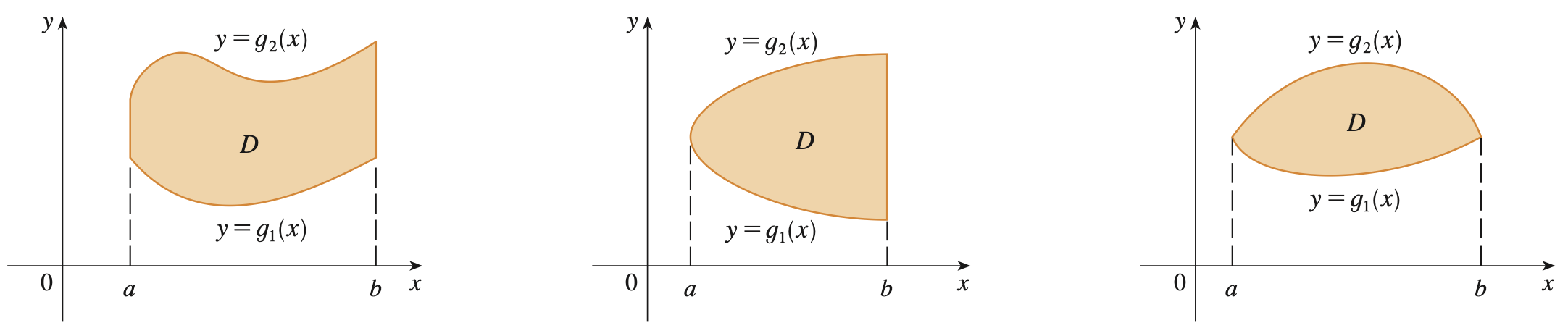
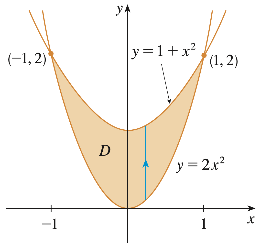
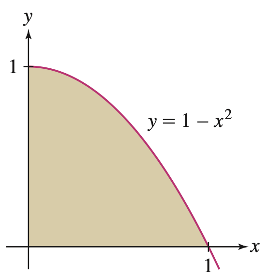
Vertically Simple: To express the domain as a vertically simple region, we bound \(x\) between two constants, and \(y\) between two functions of \(x\text{.}\) Looking at the figure, \(x\) ranges from \(0\) to \(1\text{.}\) For a given \(x\) in this interval, \(y\) goes from the \(x\)-axis (\(y = 0\)) up to the curve \(y = 1 - x^2\text{.}\)
\begin{align*} \iint_\c{D} xy \, dA \amp = \int_0^1 \int_0^{1-x^2} xy \, dy \, dx \end{align*}
Evaluating the inner integral with respect to \(y\text{:}\)
\begin{align*} \int_0^{1-x^2} xy \, dy \amp = \left[ \frac{1}{2}xy^2 \right]_{y=0}^{y=1-x^2} \\ \amp = \frac{1}{2}x(1 - x^2)^2 = \frac{1}{2}x(1 - 2x^2 + x^4) = \frac{1}{2}x - x^3 + \frac{1}{2}x^5 \end{align*}
Evaluating the outer integral with respect to \(x\text{:}\)
\begin{align*} \int_0^1 \left( \frac{1}{2}x - x^3 + \frac{1}{2}x^5 \right) \, dx \amp = \left[ \frac{1}{4}x^2 - \frac{1}{4}x^4 + \frac{1}{12}x^6 \right]_0^1 \\ \amp = \frac{1}{4} - \frac{1}{4} + \frac{1}{12} = \frac{1}{12} \end{align*}
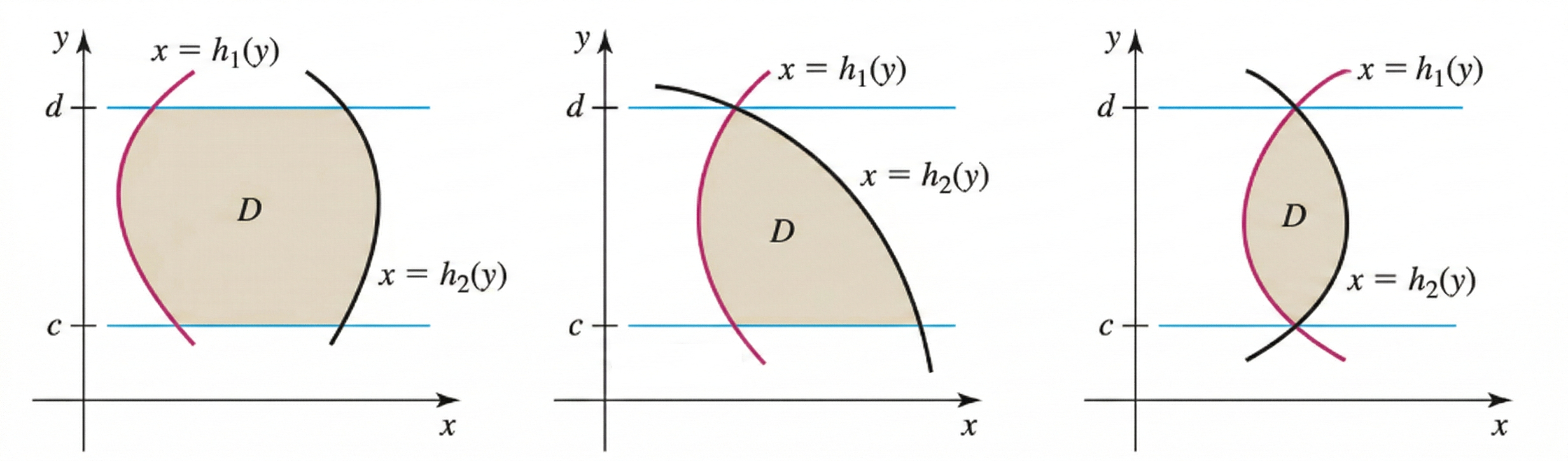
Horizontally Simple: To express it as a horizontally simple region, we bound \(y\) between two constants, and \(x\) between two functions of \(y\text{.}\) First, we solve the curve equation for \(x\text{:}\) \(y = 1 - x^2 \implies x^2 = 1 - y\text{.}\) Since we are in the first quadrant, \(x = \sqrt{1 - y}\text{.}\) \(y\) ranges from \(0\) to \(1\text{.}\) For a given \(y\text{,}\) \(x\) goes from the \(y\)-axis (\(x = 0\)) out to the curve \(x = \sqrt{1 - y}\text{.}\)
\begin{align*} \iint_\c{D} xy \, dA \amp = \int_0^1 \int_0^{\sqrt{1-y}} xy \, dx \, dy \end{align*}
Evaluating the inner integral with respect to \(x\text{:}\)
\begin{align*} \int_0^{\sqrt{1-y}} xy \, dx \amp = \left[ \frac{1}{2}x^2y \right]_{x=0}^{x=\sqrt{1-y}} \\ \amp = \frac{1}{2}(\sqrt{1-y})^2 y = \frac{1}{2}(1 - y)y = \frac{1}{2}y - \frac{1}{2}y^2 \end{align*}
Evaluating the outer integral with respect to \(y\text{:}\)
\begin{align*} \int_0^1 \left( \frac{1}{2}y - \frac{1}{2}y^2 \right) \, dy \amp = \left[ \frac{1}{4}y^2 - \frac{1}{6}y^3 \right]_0^1 \\ \amp = \frac{1}{4} - \frac{1}{6} = \frac{3}{12} - \frac{2}{12} = \frac{1}{12} \end{align*}
As expected by Fubini’s Theorem, both orders of integration yield the exact same result: \(\frac{1}{12}\text{.}\)

15.2.9.

Integrate \(f(x,y) = x\) over the region bounded by \(y = x^2\) and \(y = x + 2\text{.}\)
Solution.
First, we find the intersection points of the two curves to determine the limits of integration. Setting them equal:
\begin{align*} x^2 \amp = x + 2 \\ x^2 - x - 2 \amp = 0 \\ (x - 2)(x + 1) \amp = 0 \implies x = 2, \text{ or } x = -1 \end{align*}
So, \(x\) ranges from \(-1\) to \(2\text{.}\) On this interval, the line \(y = x + 2\) is above the parabola \(y = x^2\text{.}\) This forms a vertically simple region.
We set up the iterated integral:
\begin{align*} \iint_\c{D} x \, dA \amp = \int_{-1}^2 \int_{x^2}^{x+2} x \, dy \, dx \end{align*}
Evaluate the inner integral with respect to \(y\text{:}\)
\begin{align*} \int_{x^2}^{x+2} x \, dy \amp = \Big[ xy \Big]_{y=x^2}^{y=x+2} \\ \amp = x(x + 2) - x(x^2) = x^2 + 2x - x^3 \end{align*}
Evaluate the outer integral with respect to \(x\text{:}\)
\begin{align*} \int_{-1}^2 (x^2 + 2x - x^3) \, dx \amp = \left[ \frac{1}{3}x^3 + x^2 - \frac{1}{4}x^4 \right]_{-1}^2 \\ \amp = \left( \frac{8}{3} + 4 - \frac{16}{4} \right) - \left( -\frac{1}{3} + 1 - \frac{1}{4} \right) \\ \amp = \left( \frac{8}{3} + 4 - 4 \right) - \left( \frac{2}{3} - \frac{1}{4} \right) \\ \amp = \frac{8}{3} - \frac{5}{12} = \frac{32 - 5}{12} = \frac{27}{12} = \frac{9}{4} \end{align*}

15.2.13.

Calculate the double integral of \(f(x,y) = x + y\) over the domain \(\c{D} = \left\{(x,y) \mid x^2 + y^2 \leq 4, \, y \geq 0 \right\}\text{.}\)
Solution.
The domain \(\c{D}\) is the top half of a circle of radius 2, centered at the origin. As a vertically simple region, \(x\) ranges from \(-2\) to \(2\text{,}\) and \(y\) goes from the \(x\)-axis (\(y = 0\)) up to the upper semicircle (\(y = \sqrt{4 - x^2}\)).
Setting up the integral:
\begin{align*} \iint_\c{D} (x + y) \, dA \amp = \int_{-2}^2 \int_0^{\sqrt{4-x^2}} (x + y) \, dy \, dx \end{align*}
Evaluate the inner integral:
\begin{align*} \int_0^{\sqrt{4-x^2}} (x + y) \, dy \amp = \left[ xy + \frac{1}{2}y^2 \right]_0^{\sqrt{4-x^2}} \\ \amp = x\sqrt{4 - x^2} + \frac{1}{2}(4 - x^2) - 0 \end{align*}
Now evaluate the outer integral:
\begin{gather*} \int_{-2}^2 \left( x\sqrt{4 - x^2} + \frac{4 - x^2}{2} \right) \, dx \end{gather*}
Notice that \(x\sqrt{4 - x^2}\) is an odd function over a symmetric interval \([-2, 2]\text{,}\) so its integral is exactly 0! We only need to integrate the second part, which is an even function:
\begin{align*} \int_{-2}^2 \frac{4 - x^2}{2} \, dx \amp = 2 \int_0^2 \left( 2 - \frac{1}{2}x^2 \right) \, dx \\ \amp = 2 \left[ 2x - \frac{1}{6}x^3 \right]_0^2 \\ \amp = 2 \left( 4 - \frac{8}{6} \right) = 2 \left( \frac{24 - 8}{6} \right) = 2 \left( \frac{16}{6} \right) = \frac{16}{3} \end{align*}

Exercise Group.

In the following exercises, compute the double integral of \(f(x,y)\) over the domain \(\c{D}\) indicated.
15.2.19.
\(f(x,y) = x\, ; \qquad 0 \leq x \leq 1, \, 1 \leq y \leq e^{x^2}\)
Solution.
The domain is already set up perfectly as a vertically simple region.
\begin{gather*} \int_0^1 \int_1^{e^{x^2}} x \, dy \, dx \end{gather*}
Evaluate the inner integral:
\begin{align*} \int_1^{e^{x^2}} x \, dy \amp = \Big[ xy \Big]_{y=1}^{y=e^{x^2}} = x\left(e^{x^2} - 1\right) \end{align*}
Evaluate the outer integral using \(u\)-substitution. Let \(u = x^2\text{,}\) then \(du = 2x \, dx\text{,}\) so \(\frac{1}{2}du = x \, dx\text{.}\) The bounds remain 0 to 1.
\begin{align*} \int_0^1 x\left(e^{x^2} - 1\right) \, dx \amp = \frac{1}{2} \int_0^1 (e^u - 1) \, du \\ \amp = \frac{1}{2} \Big[ e^u - u \Big]_0^1 \\ \amp = \frac{1}{2} \big( (e^1 - 1) - (e^0 - 0) \big) \\ \amp = \frac{1}{2} (e - 1 - 1) = \frac{e - 2}{2} \end{align*}
15.2.23.
\(f(x,y) = e^{x + y} \, \qquad \text{bounded by } y = x - 1, \, y = 12 - x, \, \text{for } 2 \leq y \leq 4\text{.}\)
Solution.
The region is bounded by \(y = x - 1\) and \(y = 12 - x\) between \(y = 2\) and \(y = 4\text{.}\) Because the \(y\)-bounds are constants, this is naturally a horizontally simple region! We should express \(x\) in terms of \(y\text{:}\)
  • \(y = x - 1 \implies x = y + 1\) (Left boundary)
  • \(y = 12 - x \implies x = 12 - y\) (Right boundary)
Setting up the integral:
\begin{gather*} \int_2^4 \int_{y+1}^{12-y} e^{x+y} \, dx \, dy \end{gather*}
Evaluate the inner integral with respect to \(x\text{:}\)
\begin{align*} \int_{y+1}^{12-y} e^{x+y} \, dx \amp = \Big[ e^{x+y} \Big]_{x=y+1}^{x=12-y} \\ \amp = e^{(12-y)+y} - e^{(y+1)+y} \\ \amp = e^{12} - e^{2y+1} \end{align*}
Evaluate the outer integral with respect to \(y\text{:}\)
\begin{align*} \int_2^4 (e^{12} - e^{2y+1}) \, dy \amp = \left[ ye^{12} - \frac{1}{2}e^{2y+1} \right]_2^4 \\ \amp = \left( 4e^{12} - \frac{1}{2}e^{9} \right) - \left( 2e^{12} - \frac{1}{2}e^{5} \right) \\ \amp = 2e^{12} - \frac{1}{2}e^{9} + \frac{1}{2}e^{5} \end{align*}

15.2.27.

Consider the double integral \(\ds \int_4^9 \int_2^{\sqrt{y}} f(x,y) \, dx \, dy\text{.}\) Sketch the domain of integration and express as an iterated integral in the opposite order.
Solution.
The current bounds describe a horizontally simple region:
\begin{align*} 4 \amp \leq y \leq 9 \\ 2 \amp \leq x \leq \sqrt{y} \end{align*}
The region is bounded on the right by the parabola \(x = \sqrt{y}\) (or \(y = x^2\)), on the left by the vertical line \(x = 2\text{,}\) and on the top and bottom by \(y = 9\) and \(y = 4\text{.}\)
If we change this to a vertically simple region (reversing the order of integration to \(dy\, dx\)), we need to find the constant bounds for \(x\text{.}\) The smallest \(x\) is given by the left boundary \(x = 2\text{.}\) The largest \(x\) occurs where \(y = 9\) hits \(x = \sqrt{y}\text{,}\) which is \(x = \sqrt{9} = 3\text{.}\) So, \(2 \leq x \leq 3\text{.}\)
For a fixed \(x\) in this interval, \(y\) goes from the parabola \(y = x^2\) at the bottom, up to the horizontal line \(y = 9\) at the top. The reversed integral is:
\begin{gather*} \int_2^3 \int_{x^2}^9 f(x,y) \, dy \, dx \end{gather*}

15.2.31.

Compute the integral of \(f(x,y) = \lp \ln(y) \rp^{-1}\) over the domain \(\c{D}\) bounded by \(y = e^x\) and \(y = e^{\sqrt{x}}\text{.}\)
Hint.
Choose the order of integration that enables you to evaluate the integral.
Solution.
We are given \(f(x,y) = \frac{1}{\ln(y)}\) and boundaries \(y = e^x\) and \(y = e^{\sqrt{x}}\text{.}\) Notice that for \(0 \lt x \lt 1\text{,}\) \(\sqrt{x} \gt x\text{,}\) so \(e^{\sqrt{x}}\) is the top boundary. They intersect at \(x = 0\) (where \(y=1\)) and \(x = 1\) (where \(y=e\)).
If we set this up as a vertically simple region (\(dy \, dx\)), we would have to integrate \(\frac{1}{\ln(y)}\) with respect to \(y\text{,}\) which does not have an elementary antiderivative. So, we must set it up as a horizontally simple region (\(dx \, dy\))!
Solving the boundaries for \(x\text{:}\)
  • \(y = e^x \implies x = \ln(y)\) (This is the right boundary)
  • \(y = e^{\sqrt{x}} \implies \sqrt{x} = \ln(y) \implies x = (\ln(y))^2\) (This is the left boundary)
Our \(y\) bounds are constants from \(y = 1\) to \(y = e\text{.}\)
Setting up and evaluating the new integral:
\begin{align*} \int_1^e \int_{(\ln(y))^2}^{\ln(y)} \frac{1}{\ln(y)} \, dx \, dy \amp = \int_1^e \left[ \frac{x}{\ln(y)} \right]_{x=(\ln(y))^2}^{x=\ln(y)} \, dy \\ \amp = \int_1^e \left( \frac{\ln(y)}{\ln(y)} - \frac{(\ln(y))^2}{\ln(y)} \right) \, dy \\ \amp = \int_1^e (1 - \ln(y)) \, dy \end{align*}
Using Integration by Parts for \(\ln(y)\) (recall \(\int \ln(y) dy = y\ln(y) - y\)):
\begin{align*} \int_1^e (1 - \ln(y)) \, dy \amp = \Big[ y - (y\ln(y) - y) \Big]_1^e \\ \amp = \Big[ 2y - y\ln(y) \Big]_1^e \\ \amp = (2e - e\ln(e)) - (2(1) - 1\ln(1)) \\ \amp = (2e - e) - (2 - 0) = e - 2 \end{align*}

15.2.35.

Consider the double integral \(\ds \int_0^1 \int_{y = x}^1 xe^{y^3} \, dy \, dx\text{.}\) Sketch the domain of integration. Then change the order of integration and evaluate. Explain the simplification achieved by changing the order.
Solution.
The current bounds are:
\begin{align*} 0 \amp \leq x \leq 1 \\ x \amp \leq y \leq 1 \end{align*}
This represents a triangle bounded by \(y = x\text{,}\) \(y = 1\text{,}\) and the \(y\)-axis (\(x = 0\)).
Integrating \(xe^{y^3}\) with respect to \(y\) first is impossible because \(e^{y^3}\) lacks the \(y^2\) term needed for a \(u\)-substitution.
Changing the order of integration to \(dx\, dy\text{,}\) we view it as a horizontally simple region. The \(y\)-values range from \(0\) to \(1\text{.}\) For a fixed \(y\text{,}\) the \(x\)-values go from the \(y\)-axis (\(x = 0\)) to the line \(x = y\text{.}\)
\begin{gather*} \int_0^1 \int_0^y xe^{y^3} \, dx \, dy \end{gather*}
Evaluate the inner integral:
\begin{align*} \int_0^y xe^{y^3} \, dx \amp = \left[ \frac{1}{2}x^2e^{y^3} \right]_{x=0}^{x=y} = \frac{1}{2}y^2e^{y^3} \end{align*}
Now, the outer integral is perfectly set up for \(u\)-substitution! Let \(u = y^3\text{,}\) then \(du = 3y^2 \, dy\text{,}\) so \(\frac{1}{6}du = \frac{1}{2}y^2 \, dy\text{.}\)
\begin{align*} \int_0^1 \frac{1}{2}y^2e^{y^3} \, dy \amp = \frac{1}{6} \int_0^1 e^u \, du \\ \amp = \frac{1}{6} \Big[ e^u \Big]_0^1 = \frac{e - 1}{6} \end{align*}
Explanation: By integrating with respect to \(x\) first, we naturally generated the \(y^2\) term required to successfully perform \(u\)-substitution on the \(e^{y^3}\) term in the outer integral.

15.2.41.

Calculate the double integral of \(f(x,y) = \dfrac{x}{y^2}\) over the triangle indicated in the following figure.
Figure 15.2.17.
Solution.
To integrate over the given triangle, we first need to determine the equations of the lines forming its boundaries. Looking at the figure, the vertices of the triangle are \((1,2)\text{,}\) \((5,2)\text{,}\) and \((3,4)\text{.}\)
Notice that if we treat this as a vertically simple region, the top boundary changes at \(x = 3\text{,}\) meaning we would have to split the integral into two pieces. However, treating it as a horizontally simple region is much easier because the left and right boundaries are consistent from the bottom (\(y=2\)) to the top (\(y=4\)).
Let’s find the equations for the left and right boundaries in terms of \(y\text{:}\)
  • Left boundary (line through \((1,2)\) and \((3,4)\)): Slope \(m = \frac{4-2}{3-1} = 1\text{.}\) Point-slope form gives \(y - 2 = 1(x - 1) \implies y = x + 1\text{.}\) Solving for \(x\text{,}\) we get \(x = y - 1\text{.}\)
  • Right boundary (line through \((5,2)\) and \((3,4)\)): Slope \(m = \frac{4-2}{3-5} = -1\text{.}\) Point-slope form gives \(y - 2 = -1(x - 5) \implies y = -x + 7\text{.}\) Solving for \(x\text{,}\) we get \(x = 7 - y\text{.}\)
Setting this up as a horizontally simple region, \(y\) goes from \(2\) to \(4\text{,}\) and \(x\) goes from \(y - 1\) to \(7 - y\text{:}\)
\begin{align*} \iint_\c{D} \frac{x}{y^2} \, dA \amp = \int_2^4 \int_{y-1}^{7-y} x y^{-2} \, dx \, dy \end{align*}
Evaluate the inner integral with respect to \(x\) (treating \(y^{-2}\) as a constant):
\begin{align*} \int_{y-1}^{7-y} x y^{-2} \, dx \amp = y^{-2} \left[ \frac{1}{2}x^2 \right]_{x=y-1}^{x=7-y} \\ \amp = \frac{1}{2y^2} \Big( (7 - y)^2 - (y - 1)^2 \Big) \\ \amp = \frac{1}{2y^2} \Big( (49 - 14y + y^2) - (y^2 - 2y + 1) \Big) \\ \amp = \frac{1}{2y^2} (48 - 12y) = \frac{24}{y^2} - \frac{6}{y} \end{align*}
Evaluate the outer integral with respect to \(y\text{:}\)
\begin{align*} \int_2^4 \left( 24y^{-2} - 6y^{-1} \right) \, dy \amp = \Big[ -24y^{-1} - 6\ln|y| \Big]_2^4 \\ \amp = \left( -\frac{24}{4} - 6\ln(4) \right) - \left( -\frac{24}{2} - 6\ln(2) \right) \\ \amp = (-6 - 6\ln(4)) - (-12 - 6\ln(2)) \\ \amp = 6 - 6\ln(4) + 6\ln(2) \end{align*}
We can simplify the natural logarithms. Since \(\ln(4) = \ln(2^2) = 2\ln(2)\text{:}\)
\begin{align*} 6 - 6(2\ln(2)) + 6\ln(2) \amp = 6 - 12\ln(2) + 6\ln(2) \\ \amp = 6 - 6\ln(2) \end{align*}
\(\text{Final Answer: } 6 - 6\ln(2)\text{.}\)

15.2.47.

Find the volume of the region bounded by \(z = 16 - y\text{,}\) \(z = y\text{,}\) \(y = x^2\text{,}\) and \(y = 8 - x^2\text{.}\)
Solution.
The volume is the double integral of the "top surface" minus the "bottom surface" over the region \(\c{D}\text{.}\) The top surface is \(z = 16 - y\) and the bottom surface is \(z = y\text{.}\) Thus, the height of our solid is \(h(x,y) = (16 - y) - y = 16 - 2y\text{.}\)
The region \(\c{D}\) on the \(xy\)-plane is bounded by \(y = x^2\) and \(y = 8 - x^2\text{.}\) We find their intersection to get our \(x\)-bounds:
\begin{align*} x^2 \amp = 8 - x^2 \\ 2x^2 \amp = 8 \implies x^2 = 4 \implies x = \pm 2 \end{align*}
So, \(x\) goes from \(-2\) to \(2\text{.}\) The parabola \(y = 8 - x^2\) opens downward and is above \(y = x^2\) on this interval.
Setting up the integral:
\begin{align*} V \amp = \int_{-2}^2 \int_{x^2}^{8-x^2} (16 - 2y) \, dy \, dx \end{align*}
Evaluate the inner integral:
\begin{align*} \int_{x^2}^{8-x^2} (16 - 2y) \, dy \amp = \Big[ 16y - y^2 \Big]_{y=x^2}^{y=8-x^2} \\ \amp = \Big( 16(8 - x^2) - (8 - x^2)^2 \Big) - \Big( 16(x^2) - (x^2)^2 \Big) \\ \amp = \Big( 128 - 16x^2 - (64 - 16x^2 + x^4) \Big) - \Big( 16x^2 - x^4 \Big) \\ \amp = (64 - x^4) - (16x^2 - x^4) \\ \amp = 64 - 16x^2 \end{align*}
Evaluate the outer integral:
\begin{align*} \int_{-2}^2 (64 - 16x^2) \, dx \amp = \left[ 64x - \frac{16}{3}x^3 \right]_{-2}^2 \\ \amp = \left( 128 - \frac{128}{3} \right) - \left( -128 + \frac{128}{3} \right) \\ \amp = 256 - \frac{256}{3} = \frac{768 - 256}{3} = \frac{512}{3} \end{align*}

15.2.53.

Calculate the average value of \(f(x,y) = e^{x + y}\) on the square domain \([0,1] \times [0,1]\text{.}\)
Solution.
The average value of a function over a region is given by \(\frac{1}{\text{Area of } \c{D}} \iint_\c{D} f(x,y) \, dA\text{.}\) The area of the square domain \(\c{D} = [0,1] \times [0,1]\) is simply \(1 \cdot 1 = 1\text{.}\)
Now we evaluate the double integral using an iterated integral. Let’s integrate with respect to \(y\) first:
\begin{align*} \iint_\c{D} e^{x+y} \, dA \amp = \int_0^1 \int_0^1 e^{x+y} \, dy \, dx \end{align*}
Evaluate the inner integral with respect to \(y\) (treating \(x\) as a constant):
\begin{align*} \int_0^1 e^{x+y} \, dy \amp = \Big[ e^{x+y} \Big]_{y=0}^{y=1} \\ \amp = e^{x+1} - e^{x+0} \\ \amp = e^{x+1} - e^x \end{align*}
Substitute this back into the outer integral and integrate with respect to \(x\text{:}\)
\begin{align*} \int_0^1 (e^{x+1} - e^x) \, dx \amp = \Big[ e^{x+1} - e^x \Big]_0^1 \\ \amp = (e^{1+1} - e^1) - (e^{0+1} - e^0) \\ \amp = (e^2 - e) - (e - 1) \\ \amp = e^2 - 2e + 1 \end{align*}
Notice that \(e^2 - 2e + 1\) can be factored into a perfect square, \((e - 1)^2\text{.}\) Since the area of the region is 1, the average value is exactly \((e - 1)^2\text{.}\)

15.2.55.

Find the average height of the "ceiling" in the figure below defined by \(z = y^2\sin(x)\) for \(0 \leq x \leq \pi\) and \(0 \leq y \leq 1\text{.}\)
Figure 15.2.18.
Solution.
First, we find the area of the rectangular domain \(\c{D} = [0,\pi] \times [0,1]\text{:}\)
\begin{gather*} \text{Area} = (\pi - 0)(1 - 0) = \pi \end{gather*}
Next, we evaluate the double integral of the height function \(z = y^2\sin(x)\) over this domain. Let’s set it up to integrate with respect to \(y\) first:
\begin{align*} \iint_\c{D} y^2\sin(x) \, dA \amp = \int_0^\pi \int_0^1 y^2\sin(x) \, dy \, dx \end{align*}
Evaluate the inner integral with respect to \(y\) (treating \(x\) as a constant):
\begin{align*} \int_0^1 y^2\sin(x) \, dy \amp = \left[ \frac{1}{3}y^3\sin(x) \right]_{y=0}^{y=1} \\ \amp = \frac{1}{3}(1)^3\sin(x) - \frac{1}{3}(0)^3\sin(x) \\ \amp = \frac{1}{3}\sin(x) \end{align*}
Substitute this back into the outer integral and integrate with respect to \(x\text{:}\)
\begin{align*} \int_0^\pi \frac{1}{3}\sin(x) \, dx \amp = \left[ -\frac{1}{3}\cos(x) \right]_0^\pi \\ \amp = -\frac{1}{3}\cos(\pi) - \left(-\frac{1}{3}\cos(0)\right) \\ \amp = -\frac{1}{3}(-1) + \frac{1}{3}(1) \\ \amp = \frac{1}{3} + \frac{1}{3} = \frac{2}{3} \end{align*}
The total volume under the ceiling is \(\frac{2}{3}\text{.}\) Finally, divide the volume by the area to find the average height:
\begin{gather*} \text{Average height} = \frac{\text{Volume}}{\text{Area}} = \frac{2/3}{\pi} = \frac{2}{3\pi} \end{gather*}