
Section 12.3 Dot Product and the Angle Between Two Vectors

So far, our operations on vectors (addition and scalar multiplication) have resulted in new vectors. But what if we want to β€œmultiply” two vectors together? It turns out there isn’t just one way to do this.
In this section, we introduce the dot product (also known as the scalar product). The dot product of two vectors will tell us how much is one vector pointing in the same direction as another.

Subsection Dot Product

Without further ado, we define the dot product of two vectors as follows:

Definition 12.3.1. Dot Product.

The dot product \(\boldsymbol{\v{v} \cdot \v{w}}\) of two vectors
\begin{equation*} \v{v} = \la v_1, v_2, v_3 \ra \, , \qquad \v{w} = \la w_1, w_2, w_3 \ra \end{equation*}
is the scalar defined by
\begin{equation*} \v{v} \cdot \v{w} = v_1 w_1 + v_2 w_2 + v_3 w_3 \end{equation*}

Note 12.3.2. You may heard of the dot product in linear algebra before....

You may hear of the term inner product if you took a linear algebra class before. The dot product is a specific example of an inner product defined on \(\R^n\) (called the standard inner product).
Let \(\v{v}, \v{w} \in \R^3\) be two vectors defined as
\begin{equation*} \v{v} = \begin{pmatrix} v_1 \\ v_2 \\ v_3 \end{pmatrix} \, , \qquad \v{w} = \begin{pmatrix} w_1 \\ w_2 \\ w_3 \end{pmatrix} \end{equation*}
Then the standard inner product of \(\v{v}\) and \(\v{w}\) , denoted by \(\v{v} \cdot \v{w}\text{,}\) is defined as
\begin{equation*} \v{v} \cdot \v{w} = \v{v}^T \v{w} = \begin{pmatrix} v_1 \amp v_2 \amp v_3 \end{pmatrix} \begin{pmatrix} w_1 \\ w_2 \\ w_3 \end{pmatrix} = v_1 w_1 + v_2 w_2 + v_3 w_3 \end{equation*}
This section is highly similar to what you may have learned about the inner product in linear algebra. In addition to the theoretical aspects, we will also focus on applications of the dot product in physics.
Observe that we can find the dot product of two vectors by multiplying their corresponding components and adding the results. This is true in \(\R^2\) (or \(\R^n\) in general) as well.
Remember that the dot product of two vectors results in a scalar (a real number) and not another vector. The dot product has several useful properties that we summarize in the following theorem.

Proof(ish) of the above theorem.

The proofs of the properties are pretty straightforward using the definition of the dot product. Richard will prove some of them in \(\R^3\) and leave the rest as exercises for you to verify (especially if you are thinking about majoring in math). You may also want to see if you are convinced that Richard’s proofs can be generalized to \(\R^n\text{.}\)
  1. Let \(\v{v} = \la v_1, v_2, v_3 \ra\text{.}\) Then
    \begin{equation*} \v{0} \cdot \v{v} = 0 \cdot v_1 + 0 \cdot v_2 + 0 \cdot v_3 = 0 \end{equation*}
  2. Let \(\v{v} = \la v_1, v_2, v_3 \ra\) and \(\v{w} = \la w_1, w_2, w_3 \ra\text{.}\) Then
    \begin{align*} \v{v} \cdot \v{w} \amp= v_1 w_1 + v_2 w_2 + v_3 w_3 \\ \amp= w_1 v_1 + w_2 v_2 + w_3 v_3 \\ \amp= \v{w} \cdot \v{v} \end{align*}
  3. The proof is left as an exercise for the reader.
  4. The proof is left as an exercise for the reader.
  5. Let \(\v{v} = \la v_1, v_2, v_3 \ra\text{.}\) Then
    \begin{equation*} \v{v} \cdot \v{v} = v_1^2 + v_2^2 + v_3^2 = \|\v{v}\|^2 \end{equation*}
Using these properties, we can prove some cool results! For example, do you know that the sum of the squares of the lengths of the four sides of a parallelogram is equal to the sum of the squares of the lengths of its two diagonals? This is also known as the parallelogram law.

Example 12.3.6.

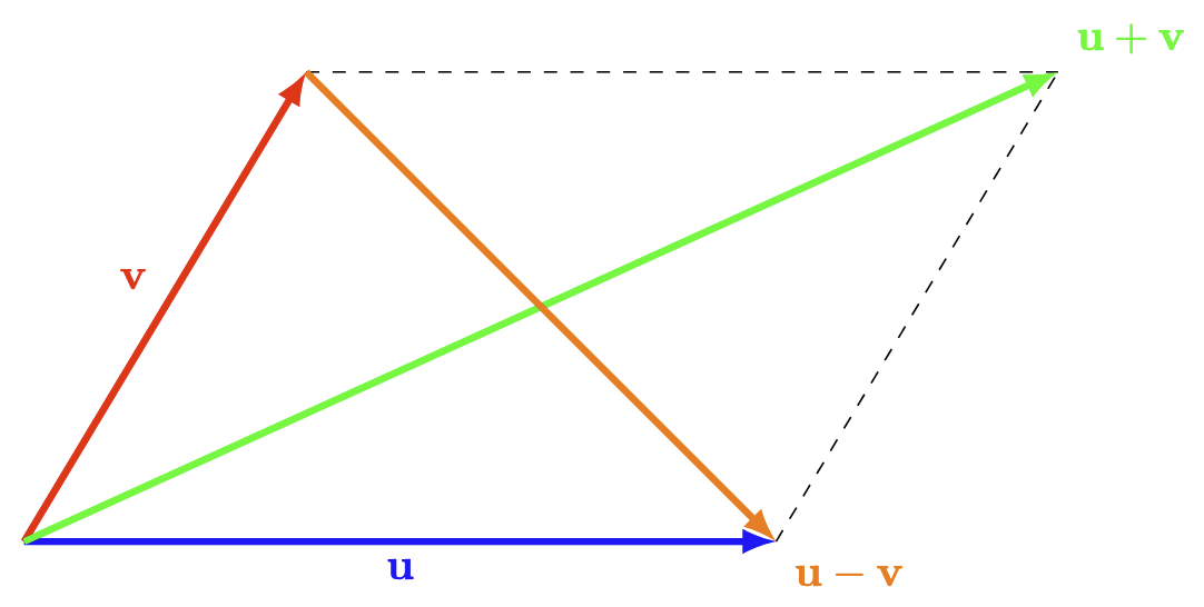
Prove the parallelogram law using the properties of the dot product. The diagram below shows a parallelogram formed by the vectors \(\v{u}\) and \(\v{v}\text{.}\)
Figure 12.3.7. Parallelogram formed by vectors \(\v{u}\) and \(\v{v}\)
Hint.
The parallelogram has two diagonals with the lengths of \(\|\v{u} + \v{v}\|\) and \(\|\v{u} - \v{v}\|\text{.}\) Also, the sides have lengths of \(\|\v{u}\|\) and \(\|\v{v}\|\text{,}\) respectively.
We are learning about the dot product so let’s get some dot products involved! One of the dot product properties states that \(\|\v{v}\|^2 = \v{v} \cdot \v{v}\) so converting all the lengths into dot products is a good start!
Solution.
\begin{align*} \|\v{u} + \v{v}\|^2 + \|\v{u} - \v{v}\|^2 \amp= (\v{u} + \v{v}) \cdot (\v{u} + \v{v}) + (\v{u} - \v{v}) \cdot (\v{u} - \v{v}) \\ \amp= \v{u} \cdot \v{u} + 2\v{u} \cdot \v{v} + \v{v} \cdot \v{v} + \v{u} \cdot \v{u} - 2\v{u} \cdot \v{v} + \v{v} \cdot \v{v} \\ \amp= 2\v{u} \cdot \v{u} + 2\v{v} \cdot \v{v} \\ \amp= 2\|\v{u}\|^2 + 2\|\v{v}\|^2 \end{align*}
Now that we know what the dot product is and some of its properties, we will next explore why we care about it.

Subsection Angle between Two Vectors

Given two vectors, they form an angle between them. But how do we know how big this angle is? The dot product can help us figure this out!
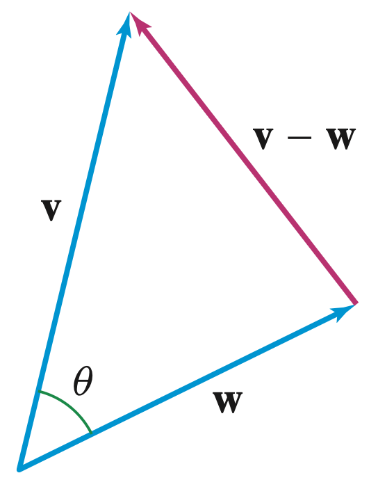
Let’s say we have two vectors, \(\v{v}\) and \(\v{w}\text{.}\) We call the angle between them \(\theta\) and we can construct the vector \(\v{v} - \v{w}\) as shown below:
Figure 12.3.8. Vectors \(\v{v}\) and \(\v{w}\) with angle \(\theta\) between them
This is essentially a triangle if we drop all the direction arrows. That is, this triangle has sides of lengths \(\|\v{v}\|\text{,}\) \(\|\v{w}\|\text{,}\) and \(\|\v{v} - \v{w}\|\text{.}\)
A relation between the sides of the triangle and the angle \(\theta\) is given by the Law of Cosines as follows:
\begin{equation*} \|\v{v} - \v{w}\|^2 = \|\v{v}\|^2 + \|\v{w}\|^2 - 2\|\v{v}\|\|\v{w}\| \cos(\theta) \end{equation*}
Using the relation with length property of the dot product and FOIL-ing, we obtain
\begin{align*} \|\v{v} - \v{w}\|^2 \amp= (\v{v} - \v{w}) \cdot (\v{v} - \v{w}) \\ \amp= \v{v} \cdot \v{v} - 2\v{v} \cdot \v{w} + \v{w} \cdot \v{w} \\ \amp= \|\v{v}\|^2 + \|\v{w}\|^2 - 2\v{v} \cdot \v{w} \end{align*}
We essentially found two ways to represent the quantity \(\|\v{v} - \v{w}\|^2\text{.}\) Equating these two expressions together and canceling stuff, we obtain
\begin{align*} \|\v{v}\|^2 + \|\v{w}\|^2 - 2\v{v} \cdot \v{w} \amp= \|\v{v}\|^2 + \|\v{w}\|^2 - 2\|\v{v}\|\|\v{w}\| \cos(\theta) \\ \implies \qquad\qquad\qquad\qquad \v{v} \cdot \v{w} \amp= \|\v{v}\|\|\v{w}\| \cos(\theta) \end{align*}
Observe that we can now solve for the angle \(\theta\) between the two vectors by isolating \(\theta\text{:}\)
\begin{equation*} \theta = \cos^{-1} \lp \frac{\v{v} \cdot \v{w}}{\|\v{v}\| \|\v{w}\|} \rp \end{equation*}
That is, the dot product gives us a way to compute the angle between two vectors!
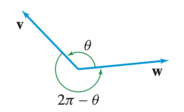
Observe that the angle is being computed using the inverse cosine function. The range of the inverse cosine function is \([0,\pi]\text{.}\) That is, we consider the angle between two vectors to be the smaller angle formed between them.
Figure 12.3.10. By convention, the angle \(\theta\) between two vectors is chosen so that \(0 \le \theta \le \pi\text{.}\)

Example 12.3.11.

Find the angle between the vectors \(\la 3,1,1 \ra\) and \(\la 2,-4,2 \ra\)
Hint.
Richard coded a fancy diagram below to help you visualize how big the angle is. The goal here is to figure out the size of \(\theta\)
Figure 12.3.12. Vectors \(\mathbf{v}=\langle 3,1,1 \rangle\) and \(\mathbf{w}=\langle 2,-4,2 \rangle\) with angle \(\theta\)
It looks like the angle between the vectors is acute...
Solution.
We denote \(\v{v} = \la 3,1,1 \ra\) and \(\v{w} = \la 2,-4,2 \ra\text{.}\) To use the formula for the cosine of the angle \(\theta\) between two vectors we need to compute the following values:
\begin{align*} \|\v{v}\| \amp= \sqrt{3^2 + 1^2 + 1^2} = \sqrt{11}\\ \|\v{w}\| \amp= \sqrt{2^2 + (-4)^2 + 2^2} = \sqrt{24}\\ \v{v} \cdot \v{w} \amp= 3 \cdot 2 + 1 \cdot (-4) + 1 \cdot 2 = 4 \end{align*}
Hence,
\begin{equation*} \cos(\theta) = \frac{\v{v} \cdot \v{w}}{\|\v{v}\| \|\v{w}\|} = \frac{4}{\sqrt{11} \cdot \sqrt{24}} = \frac{2}{\sqrt{66}} \end{equation*}
and so,
\begin{equation*} \theta = \cos^{-1} \lp \frac{2}{\sqrt{66}} \rp \approx 1.322 \end{equation*}
The angle \(\theta\) is approximately \(76^\circ\text{,}\) which is indeed acute.

Example 12.3.13.

Find the angle between the vectors \(\la 0,1,1 \ra\) and \(\la 1,-1,0 \ra\)
Hint.
Richard coded a fancy diagram below to help you visualize how big the angle is. The goal here is to figure out the size of \(\theta\)
Figure 12.3.14. Vectors \(\mathbf{v}=\langle 0,1,1 \rangle\) and \(\mathbf{w}=\langle 1,-1,0 \rangle\) with angle \(\theta\)
It looks like the angle between the vectors is obtuse...
Solution.
We denote \(\v{v} = \la 0,1,1 \ra\) and \(\v{w} = \la 1,-1,0 \ra\text{.}\) To use the formula for the cosine of the angle \(\theta\) between two vectors we need to compute the following values:
\begin{align*} \|\v{v}\| \amp= \sqrt{0^2 + 1^2 + 1^2} = \sqrt{2}\\ \|\v{w}\| \amp= \sqrt{1^2 + (-1)^2 + 0^2} = \sqrt{2}\\ \v{v} \cdot \v{w} \amp= 0 \cdot 1 + 1 \cdot (-1) + 1 \cdot 0 = -1 \end{align*}
Hence,
\begin{equation*} \cos(\theta) = \frac{\v{v} \cdot \v{w}}{\|\v{v}\| \|\v{w}\|} = \frac{-1}{\sqrt{2} \cdot \sqrt{2}} = -\frac{1}{2} \end{equation*}
and so,
\begin{equation*} \theta = \cos^{-1} \lp -\frac{1}{2} \rp = \frac{2\pi}{3} = \frac{2\pi}{3} \end{equation*}
The angle \(\theta\) is \(120^\circ\text{,}\) which is indeed obtuse.

Example 12.3.15.

Find the angle between the vectors \(\la 1,1,-1 \ra\) and \(\la 1,-2,-1 \ra\)
Hint.
Richard coded a fancy diagram below to help you visualize how big the angle is. The goal here is to figure out the size of \(\theta\)
Figure 12.3.16. Vectors \(\mathbf{v}=\langle 1,1,-1 \rangle\) and \(\mathbf{w}=\langle 1,-2,-1 \rangle\) with angle \(\theta\)
It looks like the angle between the vectors is a right angle...
Solution.
We denote \(\v{v} = \la 1,1,-1 \ra\) and \(\v{w} = \la 1,-2,-1 \ra\text{.}\) To use the formula for the cosine of the angle \(\theta\) between two vectors we need to compute the following values:
\begin{align*} \|\v{v}\| \amp= \sqrt{1^2 + 1^2 + (-1)^2} = \sqrt{3}\\ \|\v{w}\| \amp= \sqrt{1^2 + (-2)^2 + (-1)^2} = \sqrt{6}\\ \v{v} \cdot \v{w} \amp= 1 \cdot 1 + 1 \cdot (-2) + (-1) \cdot (-1) = 0 \end{align*}
Hence,
\begin{equation*} \cos(\theta) = \frac{\v{v} \cdot \v{w}}{\|\v{v}\| \|\v{w}\|} = \frac{0}{\sqrt{3} \cdot \sqrt{6}} = 0 \end{equation*}
and so,
\begin{equation*} \theta = \cos^{-1}(0) = \frac{\pi}{2} \end{equation*}
The angle \(\theta\) is \(90^\circ\text{,}\) which is indeed a right angle.
We can find a pattern from the above examples.
  • If the dot product is positive, then the angle between the vectors is acute.
  • If the dot product is negative, then the angle between the vectors is obtuse.
  • If the dot product is zero, then the angle between the vectors is a right angle.
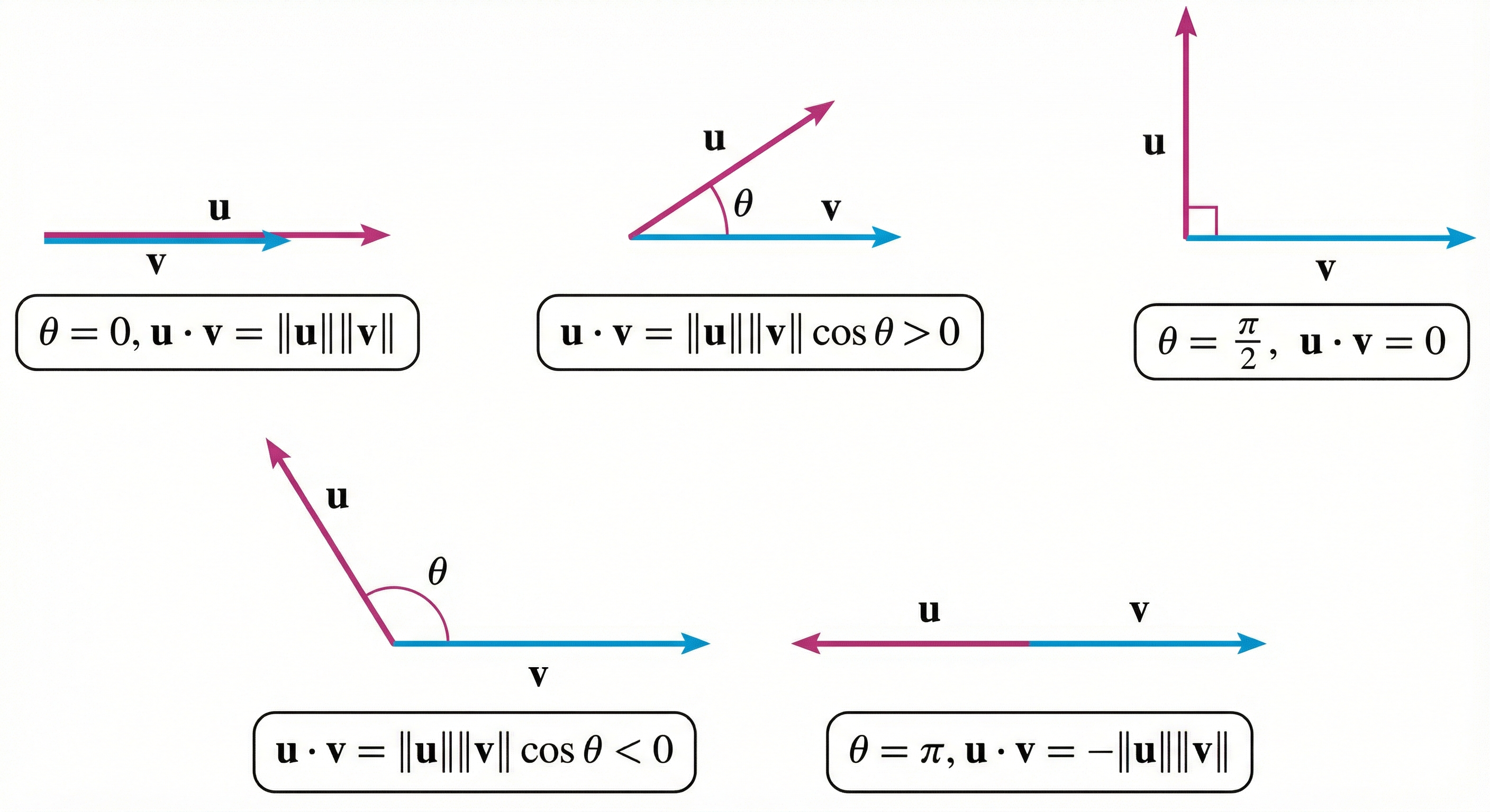
This is true since we know that \(\cos(\theta)\) is positive for acute angles, negative for obtuse angles, and zero for right angles. In addition, \(\cos(\theta) = 1\) when \(\theta = 0^\circ\) and \(\cos(\theta) = -1\) when \(\theta = 180^\circ\text{.}\) Let’s summarize this in a nice little diagram.
Figure 12.3.17. Relation between the dot product and the angle between two vectors
This diagram is really demonstrating the famous Cauchy-Schwarz Inequality, which states that the absolute value of the dot product of two vectors is always less than or equal to the product of their individual lengths. Symbolically, this is stated as
\begin{equation*} |\v{v} \cdot \v{w}| \le \|\v{v}\| \|\v{w}\| \end{equation*}
Observe from the figure that \(-1 \lt \cos(\theta) \lt 1\text{,}\) so \(\v{u} \cdot \v{v}\text{,}\) which equals to \(\|\v{u}\| \|\v{v}\| \cos(\theta)\text{,}\) cannot be greater than \(\|\v{u}\| \|\v{v}\|\text{.}\)

Example 12.3.18.

Prove the triangle inequality: For any vectors \(\v{u}\) and \(\v{v}\text{,}\)
\begin{equation*} \|\v{u} + \v{v}\| \le \|\v{u}\| + \|\v{v}\| \end{equation*}
Hint.
Of course you can draw a picture to see why this is true but this way isn’t rigorous enough. True story, one of Richard’s students tried to prove the inequality by drawing a loosey-goosey triangle and "eyeballing" the lengths of the sides of the triangle... Not rigorous at all...
Also, just because the inequality holds for one triangle doesn’t mean it holds for all triangles!
We want to show that this inequality is true for ALL triangles without relying on the accuracy of a drawing. Relying on definitions, properties, theorems, and algebraic manipulations is a better way to go!
Richard will help you get started. We are learning about the dot product so let’s get some dot products involved! One of the dot product properties states that \(\|\v{v}\|^2 = \v{v} \cdot \v{v}\) so converting all the lengths into dot products is a good start!
Also, ... where does the inequality come from? Well the Cauchy Schwarz Inequality involves an inequality! Maybe we can use that somewhere...
Solution.
\begin{align*} \|\v{u} + \v{v}\|^2 \amp= (\v{u} + \v{v}) \cdot (\v{u} + \v{v}) \\ \amp= \v{u} \cdot \v{u} + 2 \v{u} \cdot \v{v} + \v{v} \cdot \v{v} \amp\amp \text{FOIL-ing} \\ \amp\le \|\v{u}\|^2 + 2 | \v{u} \cdot \v{v} | + \|\v{v}\|^2 \\ \amp\le \|\v{u}\|^2 + 2 \|\v{u}\| \|\v{v}\| + \|\v{v}\|^2 \amp\amp \text{Cauchy-Schwarz} \\ \amp= (\|\v{u}\| + \|\v{v}\|)^2 \end{align*}
The triangle inequality follows immediately by taking the square root of both sides.
Observe that the dot product is zero when two vectors are orthogonal (or perpendicular) to each other. This is how we define orthogonality in general.

Definition 12.3.19. Orthogonal Vectors.

Two vectors \(\v{v}\) and \(\v{w}\) are orthogonal if and only if \(\v{v} \cdot \v{w} = 0\text{.}\) We denote this by \(\v{v} \perp \v{w}\text{.}\)
Based on this definition, we see that the zero vector is orthogonal to every vector since the dot product with the zero vector is always zero.

Note 12.3.20. But Richard... Isn’t "orthogonal" just another fancy way of saying perpendicular?

Yes and no... They are for sure describing the same idea but with some subtle differences.
Perpendicularity/Perpendicular is a geometric term that describes two things (like lines, planes, etc.) intersect at a right angle (90Β°). This idea only makes sense in a geometric context where we can visualize angles.
Orthogonality/Orthogonal is an algebraic term that describes two vectors whose dot product is zero. This idea makes sense in any dimension and doesn’t rely on visualizing angles. For example, the zero vector is orthogonal to every vector but it doesn’t make sense to say that the zero vector is perpendicular to every vector since the zero vector doesn’t have a length (we don’t say a point is perpendicular to a line).
Surprise surprise, there is another term that describes the same idea in math: normality/normal. Normality is often used to describe things that are orthogonal/perpendicular to a surface/plane/line. For example, a normal vector to a plane is a vector that is orthogonal to every vector lying in that plane.

Example 12.3.21.

Determine whether the following vectors are orthogonal and, if not, whether the angle between them is acute or obtuse.
  1. \(\la 1,2,1 \ra\) and \(\la 7,-3,-1 \ra\)
  2. \(\la 0,2,4 \ra\) and \(\la 3,1,0 \ra\)
  3. \(\la \dfrac{12}{5}, -\dfrac{4}{5} \ra\) and \(\la \dfrac{1}{2}, \dfrac{7}{4} \ra\)
Solution.
We can determine whether the vectors are orthogonal by computing their dot products.
  1. Observe that
    \begin{equation*} \la 1,2,1 \ra \cdot \la 7,-3,-1 \ra = 1\cdot 7 + 2\cdot (-3) + 1\cdot (-1) = 7 - 6 - 1 = 0\text{.} \end{equation*}
    Therefore, the vectors are orthogonal.
  2. Observe that
    \begin{equation*} \la 0,2,4 \ra \cdot \la 3,1,0 \ra = 0\cdot 3 + 2\cdot 1 + 4\cdot 0 = 0 + 2 + 0 = 2\text{.} \end{equation*}
    Since the dot product is positive, the angle between the vectors is acute.
  3. Observe that
    \begin{equation*} \la \dfrac{12}{5}, -\dfrac{4}{5} \ra \cdot \la \dfrac{1}{2}, \dfrac{7}{4} \ra = -\dfrac{1}{5}\text{.} \end{equation*}
    Since the dot product is negative, the angle between the vectors is obtuse.
Remember our standard basis vectors in \(\R^3\text{?}\) These vectors are
\begin{equation*} \v{i} = \la 1,0,0 \ra\, , \qquad \v{j} = \la 0,1,0 \ra\, , \qquad \text{ and } \qquad \v{k} = \la 0,0,1 \ra\text{.} \end{equation*}
They are mutually orthogonal and have length \(1\text{.}\) So we have
\begin{equation*} \v{i} \cdot \v{j} = \v{i} \cdot \v{k} = \v{j} \cdot \v{k} = 0 \qquad \text{ and } \qquad \v{i} \cdot \v{i} = \v{j} \cdot \v{j} = \v{k} \cdot \v{k} = 1 \end{equation*}
Now we can compute the product using these basis vectors!

Example 12.3.22.

Compute the dot product \(\lp 3\v{j} + 2\v{k} \rp \cdot \lp \v{i} - 4\v{k} \rp\)
Hint.
Remember that the dot product is distributive! That is, we can FOIL this expression out like we would with regular multiplication. Then we can use the properties of the dot product with the basis vectors to simplify!
Solution.
\begin{align*} \lp 3\v{j} + 2\v{k} \rp \cdot \lp \v{i} - 4\v{k} \rp \amp= 3\v{j} \cdot \v{i} - 12\v{j} \cdot \v{k} + 2\v{k} \cdot \v{i} - 8\v{k} \cdot \v{k} \\ \amp= 3 \cdot 0 - 12 \cdot 0 + 2 \cdot 0 - 8 \cdot \|\v{k}\|^2 \\ \amp= -8 \cdot 1^2 \\ \amp= -8 \end{align*}

Subsection Orthogonal Projection

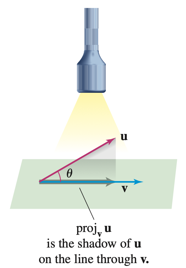
Remember that the dot product should tell us something about how much one vector goes in the direction of another vector. You may get the idea that the sign of the dot product tells us whether the vectors point in similar directions (acute angle) or opposite directions (obtuse angle). But we can actually know more! The orthogonal projection of one vector onto another vector, which is obtained using the dot product, gives us a precise way to measure how much one vector goes in the direction of another vector.
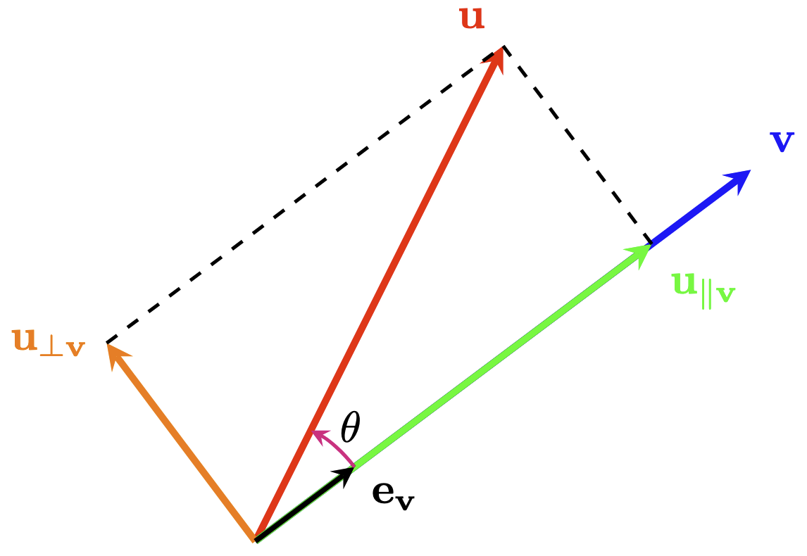
Let’s say we have two vectors \(\v{u}\) and \(\v{v}\) and we cast a shadow of \(\v{u}\) on the light through \(\v{v}\text{.}\) This shadow is called the orthogonal projection of \(\v{u}\) onto \(\v{v}\) and is denoted by \(\proj_{\v{v}} \v{u}\text{.}\)
Figure 12.3.23. The Projection of \(\v{u}\) onto \(\v{v}\)
But how do we find this projection vector? We can use the dot product to help us out!
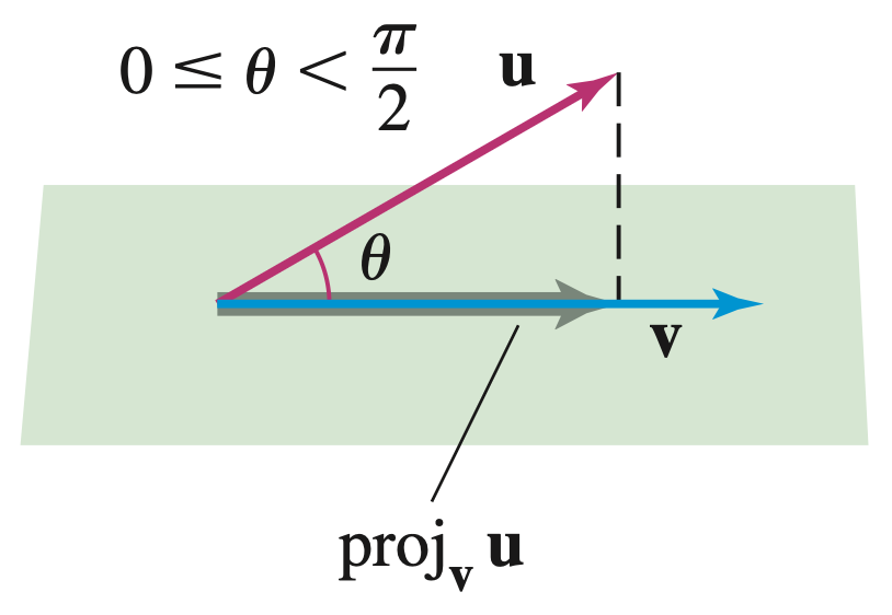
Let’s assume two vectors are pointing in the same(ish) direction, which means the angle between them is acute. The diagram is shown below and our goal is to find the length and the direction of the projection vector.
Figure 12.3.24. The Projection of \(\v{u}\) onto \(\v{v}\) with an acute angle between them
Let’s tackle the length first. Using trigonometry (and yes there is a right triangle in there somewhere that allows us to use trig), we see that the length of the projection vector is
\begin{equation*} \|\proj_{\v{v}} \v{u}\| = \|\v{u}\| \cos(\theta) \end{equation*}
Next, we need to find the direction of the projection vector. Clearly, the projection vector points in the same direction as \(\v{v}\text{.}\) Yet, we can’t just simply multiply the length by \(\v{v}\text{.}\) If we did that, the length of the projection vector would be off by a factor of \(\|\v{v}\|\text{.}\) To fix this, we use the unit vector in the direction of \(\v{v}\text{,}\) which is \(\v{e_v} = \dfrac{\v{v}}{\|\v{v}\|}\text{.}\)
Therefore, the projection vector is
\begin{align*} \proj_{\v{v}} \v{u} \amp= \|\v{u}\| \cos(\theta) \frac{\v{v}}{\|\v{v}\|} \\ \amp= \frac{\v{u} \cdot \v{v}}{\|\v{v}\|} \frac{\v{v}}{\|\v{v}\|} \\ \amp= \frac{\v{u} \cdot \v{v}}{\|\v{v}\|^2} \v{v} \\ \amp= \frac{\v{u} \cdot \v{v}}{\v{v} \cdot \v{v}} \v{v} \end{align*}
This projection vector is also denoted by \(\v{u}_{\parallel \v{v}}\) since we can think of it as the component of \(\v{u}\) that is parallel to \(\v{v}\text{.}\)

Definition 12.3.25. Projection of \(\v{u}\) onto \(\v{v}\).

Assume \(\v{v} \neq 0\text{.}\) The projection of \(\v{u}\) onto \(\v{v}\) is the vector
\begin{equation*} \v{u}_{\parallel \v{v}} = \lp \frac{\v{u} \cdot \v{v}}{\| \v{v}\|} \rp \v{e_v} = \lp \frac{\v{u} \cdot \v{v}}{\|\v{v}\|^2} \rp \v{v} = \lp \frac{\v{u} \cdot \v{v}}{\v{v} \cdot \v{v}} \rp \v{v} \end{equation*}
This is sometimes denoted by \(\proj_{\v{v}} \v{u}\text{.}\) The scalar \(\dfrac{\v{u} \cdot \v{v}}{\|\v{v}\|}\) is called the scalar component of \(\v{u}\) onto \(\v{v}\) and is sometimes denoted by \(\comp_{\v{v}} \v{u}\text{.}\)
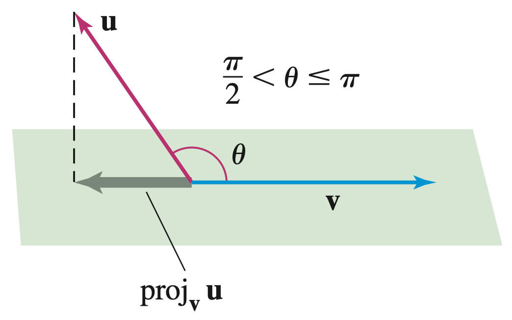
Note 12.3.26. But Richard... What if the angle between the vectors is obtuse?

The previous result was derived assuming the angle between the vectors is acute. But what if the angle is obtuse, like in the diagram below? Does the formula for the projection vector still hold?
Figure 12.3.27. The Projection of \(\v{u}\) onto \(\v{v}\) with an obtuse angle between them
The answer is yes but the work is a bit different. Richard will encourage you to try proving the formula for the projection vector in this case as an exercise.
Richard’s proof if you want to check your proof.
The work is almost identical to the acute angle case with one bit of difference.
Let \(\theta\) be an obtuse angle, which means \(\frac{\pi}{2} \lt \theta \lt \pi\text{.}\) Using trigonometry, we can find the length of the projection vector as follows:
\begin{align*} \|\proj_{\v{v}} \v{u} \| \amp= \|\v{u}\|\cos \lp \pi - \theta \rp \\ \amp= \|\v{u}\|\cdot -\cos(\theta) \\ \amp= -\|\v{u}\| \cos(\theta) \end{align*}
While there is a negative sign in front of the length, this is a positive quantity since \(\cos(\theta)\) is negative for \(\frac{\pi}{2} \lt \theta \lt \pi\text{.}\)
Next, we find the direction of the projection vector. Clearly, the projection vector points in the opposite direction as \(\v{v}\) (look at the diagram!). Then the unit vector in the direction opposite to \(\v{v}\) is \(-\dfrac{\v{v}}{\|\v{v}\|}\text{.}\)
Therefore, the projection vector is
\begin{align*} \proj_{\v{v}} \v{u} \amp= -\|\v{u}\| \cos(\theta) \lp -\frac{\v{v}}{\|\v{v}\|} \rp \\ \amp= \frac{\v{u} \cdot \v{v}}{\|\v{v}\|} \frac{\v{v}}{\|\v{v}\|} \\ \amp= \frac{\v{u} \cdot \v{v}}{\|\v{v}\|^2} \v{v} \\ \amp= \frac{\v{u} \cdot \v{v}}{\v{v} \cdot \v{v}} \v{v} \end{align*}
which is the same formula as before.
Observe that Richard didn’t bother with the case when the angle between the vectors is a right angle. This is because the projection vector is simply the zero vector in this case since \(\v{u} \cdot \v{v} = 0\text{.}\)

Example 12.3.28.

Find the projection of \(\v{u}\) onto \(\v{v}\) where \(\v{u} = \la 1,1,2 \ra\) and \(\v{v} = \la -2,3,1 \ra\text{.}\)
Hint.
To help you visualize the projection, Richard coded up the following fancy diagram:
Figure 12.3.29. Projection of \(\mathbf{u}=\langle 1,1,2 \rangle\) onto \(\mathbf{v}=\langle -2,3,1 \rangle\)
The goal is to find the green projection vector in the diagram above.
Solution.
The projection of \(\v{u}\) onto \(\v{v}\) is the following vector
\begin{equation*} \proj_{\v{v}} \v{u} = \lp \frac{\v{u} \cdot \v{v}}{\v{v} \cdot \v{v}} \rp \v{v} \end{equation*}
We compute the values in this expression:
\begin{align*} \v{u} \cdot \v{v} \amp= \la 1,1,2 \ra \cdot \la -2,3,1 \ra = 1\cdot(-2) + 1\cdot 3 + 2\cdot 1 = -2 + 3 + 2 = 3 \\ \v{v} \cdot \v{v} \amp= \la -2,3,1 \ra \cdot \la -2,3,1 \ra = (-2)^2 + 3^2 + 1^2 = 4 + 9 + 1 = 14 \end{align*}
Hence,
\begin{equation*} \proj_{\v{v}} \v{u} = \lp \frac{3}{14} \rp \la -2,3,1 \ra = \la -\frac{3}{7}, \frac{9}{14}, \frac{3}{14} \ra \end{equation*}
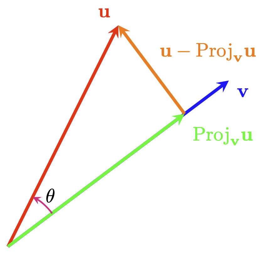
Now that we know what the projection looks like, the next question to consider is: how different is the vector from its projection? A quick subtraction \(\v{u} - \proj_{\v{v}} \v{u}\) will give us the answer.
Figure 12.3.30. Vector \(\v{u}\) (red), \(\v{v}\) (blue), \(\proj_{\v{v}} \v{u}\) (green), and \(\v{u} - \proj_{\v{v}} \v{u}\) (orange)
Observe that this difference vector is orthogonal to \(\v{v}\text{.}\) This is one way that we can decompose the vector \(\v{u}\) into two components with respect to \(\v{v}\text{:}\) one component that is parallel to \(\v{v}\) (aka the projection vector) and another component that is orthogonal to \(\v{v}\text{.}\) Remember we also denote the projection vector by \(\v{u}_{\parallel \v{v}}\) (this is sometimes referred as the parallel component). Then we can denote the difference vector by \(\v{u}_{\perp \v{v}}\) (this is sometimes referred to as the normal component).
This gives us the following decomposition of \(\v{u}\) with respect to \(\v{v}\text{:}\)
\begin{equation*} \v{u} = \v{u}_{\parallel \v{v}} + \v{u}_{\perp \v{v}} \end{equation*}
Figure 12.3.31. Vector \(\v{u}\) (red), \(\v{v}\) (blue), \(\proj_{\v{v}} \v{u}\) (green), and \(\v{u} - \proj_{\v{v}} \v{u}\) (orange)
This is actually the Orthogonal Decomposition Theorem in linear algebra.

Example 12.3.32.

Find the decomposition \(\v{u} = \v{u}_{\parallel \v{v}} + \v{u}_{\perp \v{v}}\) for the vectors \(\v{u} = \la 4,-1,5 \ra\) and \(\v{v} = \la 2,1,1 \ra\text{.}\)
Hint.
To help you visualize the decomposition, Richard coded up the following fancy diagram:
Figure 12.3.33. Decomposition of \(\v{u}\) with respect to \(\v{v}\)
The goal is to find the two components \(\v{u}_{\parallel \v{v}}\) and \(\v{u}_{\perp \v{v}}\) in the diagram above.
Solution.
We first compute \(\v{u} \cdot \v{v}\) and \(\v{v} \cdot \v{v}\) to find the projection of \(\v{u}\) onto \(\v{v}\text{:}\)
\begin{align*} \v{u} \cdot \v{v} \amp= \la 4,-1,5 \ra \cdot \la 2,1,1 \ra = 4\cdot 2 + (-1)\cdot 1 + 5\cdot 1 = 8 - 1 + 5 = 12 \\ \v{v} \cdot \v{v} \amp= \la 2,1,1 \ra \cdot \la 2,1,1 \ra = 2^2 + 1^2 + 1^2 = 4 + 1 + 1 = 6 \end{align*}
Hence,
\begin{equation*} \v{u}_{\parallel \v{v}} = \proj_{\v{v}} \v{u} = \lp \frac{12}{6} \rp \la 2,1,1 \ra = 2 \la 2,1,1 \ra = \la 4,2,2 \ra \end{equation*}
We now find the vector \(\v{u}_{\perp \v{v}}\) by computing the difference:
\begin{equation*} \v{u}_{\perp \v{v}} = \v{u} - \v{u}_{\parallel \v{v}} = \la 4,-1,5 \ra - \la 4,2,2 \ra = \la 0,-3,3 \ra \end{equation*}
Thus, we have
\begin{equation*} \v{u} = \v{u}_{\parallel \v{v}} + \v{u}_{\perp \v{v}} = \la 4,2,2 \ra + \la 0,-3,3 \ra \end{equation*}
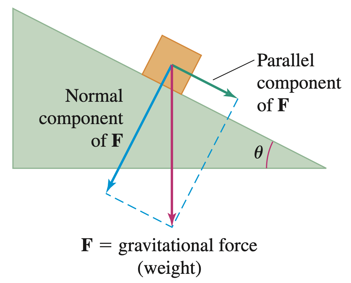
The ability to decompose vectors into orthogonal components is useful in many applications. For example, when an object rests on an inclined plane, the gravitational force acting on the object equals its weight, which is directly vertically downward. However, to analyze the motion of the object on the inclined plane, it is often helpful to decompose the gravitational force vector into two components: one parallel to the plane (which determines the tendency of the object to slide down the plane) and another perpendicular to the plane (which determines its tendency to "stick" to the plane).
Figure 12.3.34. Gravitational force decomposition on an inclined plane

Example 12.3.35.

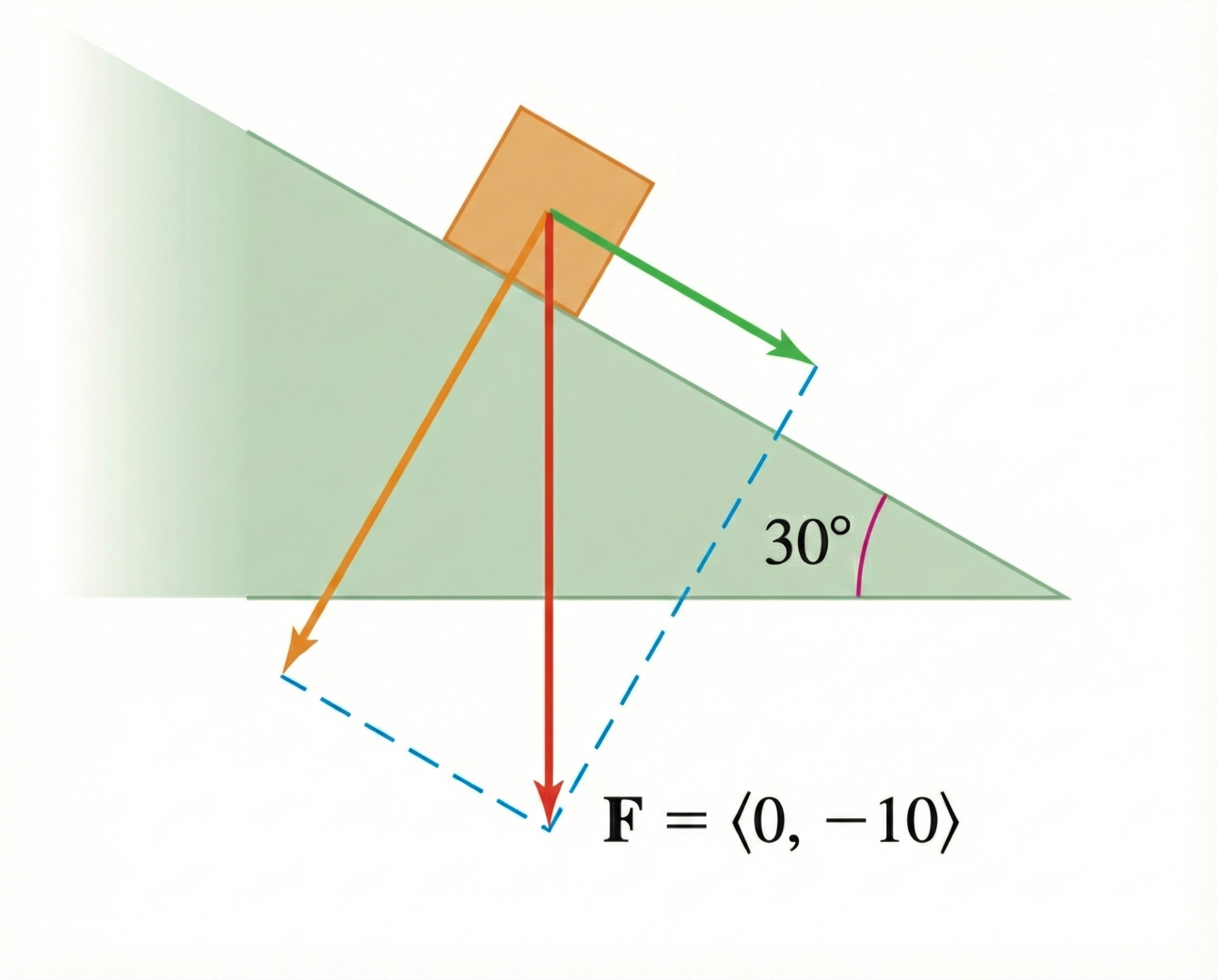
A 10-lb block rests on a plane that is inclined at 30Β° below the horizontal. Find the components of the gravitational force parallel and normal perpendicular to the plane.
Hint.
See below for the diagram of the situation:
Figure 12.3.36. Gravitational force Vector (red), Parallel Component (green), and Perpendicular Component (orange)
The goal here is to find the green and the orange vectors in the diagram above.
Solution.
The gravitational force \(\v{F}\) acting on the block equals the weight o the block. Using the coordinate system, the force acts in the negative \(y\)-direction, so
\begin{equation*} \v{F} = \la 0, -10 \ra \end{equation*}
The direction down the plane is given by the vector is
\begin{equation*} \v{v} = \la \cos(-30^\circ), \sin(-30^\circ) \ra = \la \frac{\sqrt{3}}{2}, -\frac{1}{2} \ra \end{equation*}
Hence, the component of the force parallel to the plane is
\begin{align*} \v{F}_{\parallel \v{v}} \amp= \lp \frac{\v{F} \cdot \v{v}}{\v{v} \cdot \v{v}} \rp \v{v} \\ \amp= \lp \frac{\la 0, -10 \ra \cdot \la \frac{\sqrt{3}}{2}, -\frac{1}{2} \ra}{\la \frac{\sqrt{3}}{2}, -\frac{1}{2} \ra \cdot \la \frac{\sqrt{3}}{2}, -\frac{1}{2} \ra} \rp \la \frac{\sqrt{3}}{2}, -\frac{1}{2} \ra \\ \amp= 5 \la \frac{\sqrt{3}}{2}, -\frac{1}{2} \ra \\ \amp= \la \frac{5\sqrt{3}}{2}, -\frac{5}{2} \ra \end{align*}
Next, the component of the force perpendicular to the plane is
\begin{align*} \v{F}_{\perp \v{v}} \amp= \v{F} - \v{F}_{\parallel \v{v}} \\ \amp= \la 0, -10 \ra - \la \frac{5\sqrt{3}}{2}, -\frac{5}{2} \ra \\ \amp= \la -\frac{5\sqrt{3}}{2}, -\frac{15}{2} \ra \end{align*}

Worksheet Assigned Problems for Section 12.3

The problems listed below are assigned to be included in your problem set portfolio. Note that a specific selection of these problems will also form the written homework assignments. I recommend working through all of them to ensure a solid grasp of the material. Reach out to Richard for help if you get stuck or have any questions.
The solutions will be posted after the written homework due dates. If you have any questions about your work, talk to Richard and he is happy to discuss the process with you.

12.3.11.

Compute the dot product \(\lp \v{i} + \v{j} + \v{k} \rp \cdot \lp 3\v{i} + 2\v{j} - 5\v{k} \rp\)
Solution.
We use properties of the dot product to obtain
\begin{align*} \lp \v{i} + \v{j} + \v{k} \rp \cdot \lp 3\v{i} + 2\v{j} - 5\v{k} \rp \amp= 3\v{i}\cdot \v{i} + 2\v{i} \cdot \v{j} - 5\v{i} \cdot \v{k} + 3\v{j} \cdot \v{i} + 2\v{j} \cdot \v{j} - 5\v{j} \cdot \v{k} + 3\v{k} \cdot \v{i} + 2\v{k} \cdot \v{j} - 5\v{k} \cdot \v{k} \\ \amp= 3\|\v{i}\|^2 + 2\|\v{j}\|^2 - 5\|\v{k}\|^2 \\ \amp= 3\cdot 1 + 2\cdot 1 - 5\cdot 1 \\ \amp= 0 \end{align*}

12.3.13.

Determine whether the two vectors \(\la 1,1,1 \ra\) and \(\la 1,-2,-2 \ra\) are orthogonal and, if not, whether the angle between them is acute or obtuse.
Solution.
We compute the dot product of the two vectors:
\begin{equation*} \la 1,1,1 \ra \cdot \la 1,-2,-2 \ra = 1\cdot 1 + 1\cdot (-2) + 1\cdot (-2) = 1 - 2 - 2 = -3 \end{equation*}
Since the dot product is negative, the angle between the vectors is obtuse.

12.3.25.

Find the angle bewteen the vectors \(\la 1,1,1 \ra\) and \(\la 1,0,1 \ra\text{.}\)
Solution.
We denote \(\v{v} = \la 1,1,1 \ra\) and \(\v{w} = \la 1,0,1 \ra\text{.}\) To use the formula for the cosine of the angle \(\theta\) between two vectors we need to compute the following values:
\begin{align*} \|\v{v}\| \amp= \sqrt{1^2 + 1^2 + 1^2} = \sqrt{3} \\ \|\v{w}\| \amp= \sqrt{1^2 + 0^2 + 1^2} = \sqrt{2} \\ \v{v} \cdot \v{w} \amp= 1\cdot 1 + 1\cdot 0 + 1\cdot 1 = 2 \end{align*}
Hence,
\begin{equation*} \cos(\theta) = \frac{\v{v}\cdot \v{w}}{\|\v{v}\|\|\v{w}\|} = \frac{2}{\sqrt{3}\cdot \sqrt{2}} = \frac{2}{\sqrt{6}} = \frac{\sqrt{6}}{3} \end{equation*}
and so,
\begin{equation*} \theta = \cos^{-1}\lp \frac{\sqrt{6}}{3} \rp \approx 0.615 \end{equation*}

12.3.37.

Simplify the expression \(\lp \v{v} - \v{w} \rp \cdot \v{v} + \v{v} \cdot \v{w}\)
Solution.
By properties of the dot product we obtain
\begin{align*} \lp \v{v} - \v{w} \rp \cdot \v{v} + \v{v} \cdot \v{w} \amp= \v{v} \cdot \v{v} - \v{w} \cdot \v{v} + \v{v} \cdot \v{w} \\ \amp= \|\v{v}\|^2 - \v{w} \cdot \v{v} + \v{v} \cdot \v{w} \\ \amp= \|\v{v}\|^2 \end{align*}

12.3.43.

Use the properties of the dot product to evaluate the expression \(2\v{u} \cdot \lp 3\v{u} - \v{v} \rp\text{,}\) assuming that \(\v{u} \cdot \v{v} = 2\text{,}\) \(\|\v{u}\| = 1\text{,}\) and \(\|\v{v}\| = 3\text{.}\)
Solution.
By properties of the dot product we obtain
\begin{align*} 2\v{u} \cdot \lp 3\v{u} - \v{v} \rp \amp= (2\v{u}) \cdot (3\v{u}) - (2\v{u}) \cdot \v{v} \\ \amp= 6 (\v{u}\cdot \v{u}) - 2 (\v{u} \cdot \v{v}) \\ \amp= 6 \|\v{u}\|^2 - 2 (\v{u} \cdot \v{v}) \\ \amp= 6\cdot 1^2 - 2 \cdot 2 \\ \amp= 2 \end{align*}

12.3.48.

Assume that \(\|\v{v}\| = 2\text{,}\) \(\|\v{w}\| = 3\text{,}\) and the angle between \(\v{v}\) and \(\v{w}\) is \(120^\circ\text{.}\) Determine
  1. \(\displaystyle \v{v} \cdot \v{w}\)
  2. \(\displaystyle \|2\v{v} + \v{w}\|\)
  3. \(\displaystyle \|2\v{v} - 3\v{w}\|\)
Solution.
  1. We use the relation between the dot product and the angle between two vectors to write
    \begin{equation*} \v{v} \cdot \v{w} = \|\v{v}\|\|\v{w}\| \cos(120^\circ) = 2 \cdot 3 \cdot \lp -\frac{1}{2} \rp = -3 \end{equation*}
  2. By the relation of the dot product with length and by properties of the dot product we have
    \begin{align*} \|2\v{v} + \v{w}\|^2 \amp= (2\v{v} + \v{w}) \cdot (2\v{v} + \v{w}) \\ \amp= 4(\v{v} \cdot \v) + 4(\v{v} \cdot \v{w}) + (\v{w} \cdot \v{w}) \\ \amp= 4\|\v{v}\|^2 + 4(\v{v} \cdot \v{w}) + \|\v{w}\|^2 \end{align*}
    We now substitute \(\v{v}\cdot \v{w} = -3\) from part a) and the given information, obtaining
    \begin{align*} \|2\v{v} + \v{w}\|^2 \amp= 4\cdot 2^2 + 4\cdot (-3) + 3^2 = 13 \\ \implies \qquad \|2\v{v} + \v{w}\| \amp= \sqrt{13} \approx 3.61 \end{align*}
  3. We express the length in terms of a dot product and use properties of the dot product. This gives
    \begin{align*} \|2\v{v} - 3\v{w}\|^2 \amp= (2\v{v} - 3\v{w}) \cdot (2\v{v} - 3\v{w}) \\ \amp= 4\v{v} \cdot \v{v} - 6\v{v} \cdot \v{w} - 6\v{w} \cdot \v{v} + 9\v{w} \cdot \v{w} \\ \amp= 4\|\v{v}\|^2 - 12\v{v} \cdot \v{w} + 9\|\v{w}\|^2 \end{align*}
    Substituting \(\v{v}\cdot \v{w} = -3\) from part a) and the given values yields
    \begin{align*} \|2\v{v} - 3\v{w}\|^2 \amp= 4\cdot 2^2 - 12\cdot (-3) + 9\cdot 3^2 = 133 \\ \implies \qquad \|2\v{v} - 3\v{w}\| \amp= \sqrt{133} \approx 11.53 \end{align*}

12.3.57.

Find the projection of \(\v{u}\) along \(\v{v}\text{,}\) where \(\v{u} = \la -1,2,0 \ra\) and \(\v{v} = \la 2,0,1 \ra\text{.}\)
Solution.
The projection of \(\v{u}\) along \(\v{v}\) is the following vector:
\begin{equation*} \v{u}_{\parallel \v{v}} = \lp \frac{\v{u} \cdot \v{v}}{\v{v} \cdot \v{v}} \rp \v{v} \end{equation*}
We compute the values in this expression:
\begin{align*} \v{u} \cdot \v{v} \amp= \la -1,2,0 \ra \cdot \la 2,0,1 \ra = -1 \cdot 2 + 2 \cdot 0 + 0 \cdot 1 = -2 \\ \v{v} \cdot \v{v} \amp= \|\v{v}\|^2 = 2^2 + 0^2 + 1^2 = 5 \end{align*}
Hence,
\begin{equation*} \v{u}_{\parallel \v{v}} = \frac{-2}{5} \la 2,0,1 \ra = \la -\frac{4}{5},0,-\frac{2}{5} \ra \end{equation*}

12.3.69.

Find the decomposition \(\v{a} = \v{a}_{\parallel \v{b}} + \v{a}_{\perp \v{b}}\) with respect to \(\v{b}\text{,}\) where \(\v{a} = \la 4,-1,0 \ra\) and \(\v{b} = \la 0,1,1 \ra\text{.}\)
Solution.
We first compute \(\v{a} \cdot \v{b}\) and \(\v{b} \cdot \v{b}\) to find the projection of \(\v{a}\) along \(\v{b}\text{:}\)
\begin{align*} \v{a} \cdot \v{b} \amp= \la 4,-1,0 \ra \cdot \la 0,1,1 \ra = 4\cdot 0 + (-1)\cdot 1 + 0\cdot 1 = -1 \\ \v{b} \cdot \v{b} \amp= \|\v{b}\|^2 = 0^2 + 1^2 + 1^2 = 2 \end{align*}
Hence,
\begin{equation*} \v{a}_{\parallel \v{b}} = \lp \frac{\v{a} \cdot \v{b}}{\v{b} \cdot \v{b}} \rp \v{b} = \frac{-1}{2} \la 0,1,1 \ra = \la 0,-\frac{1}{2}, -\frac{1}{2} \ra \end{equation*}
We now find the vector \(\v{a}_{\perp \v{b}}\) orthogonal to \(\v{b}\) by computing the difference:
\begin{equation*} \v{a} - \v{a}_{\perp \v{b}} = \la 4,-1,0 \ra - \la 0,-\frac{1}{2},-\frac{1}{2} \ra = \la 4,-\frac{1}{2},\frac{1}{2} \ra \end{equation*}
Thus, we have
\begin{equation*} \v{a} = \v{a}_{\parallel \v{b}} + \v{a}_{\perp \v{b}} = \la 0,-\frac{1}{2}, -\frac{1}{2} \ra + \la 4,-\frac{1}{2},\frac{1}{2} \ra \end{equation*}

12.3.75.

Find the angle between \(\overline{AB}\) and \(\overline{AC}\) in the following figure.
Figure 12.3.37. Unit cube in \(\R^3\)
Solution.
The cosine of the angle \(\alpha\) between the vectors \(\overline{AB}\) and \(\overline{AC}\) is
\begin{equation*} \cos (\alpha) = \frac{\overrightarrow{AB} \cdot \overrightarrow{AC}}{\|\overrightarrow{AB}\| \|\overrightarrow{AC}\|} \end{equation*}
We compute the vectors \(\overrightarrow{AB}\) and \(\overrightarrow{AC}\) and then calculate their dot product and lengths. We get
\begin{align*} \overrightarrow{AB} \amp= \la 1-0, 0-0, 0-1 \ra = \la 1,0,-1 \ra \\ \overrightarrow{AC} \amp= \la 1-0, 1-0, 0-1 \ra = \la 1,1,-1 \ra \\ \overrightarrow{AB} \cdot \overrightarrow{AC} \amp= \la 1,0,-1 \ra \cdot \la 1,1,-1 \ra = 1\cdot 1 + 0\cdot 1 + (-1)\cdot (-1) = 2 \\ \|\overrightarrow{AB}\| \amp= \sqrt{1^2 + 0^2 + (-1)^2} = \sqrt{2} \\ \|\overrightarrow{AC}\| \amp= \sqrt{1^2 + 1^2 + (-1)^2} = \sqrt{3} \end{align*}
Substituting these values into the formula for the cosine of the angle and solving for \(0 \le \alpha \le \pi\) gives
\begin{equation*} \cos(\alpha) = \frac{2}{\sqrt{2} \cdot \sqrt{3}} \approx 0.816 \qquad \implies \qquad \alpha \approx 0.615 \end{equation*}

12.3.85.

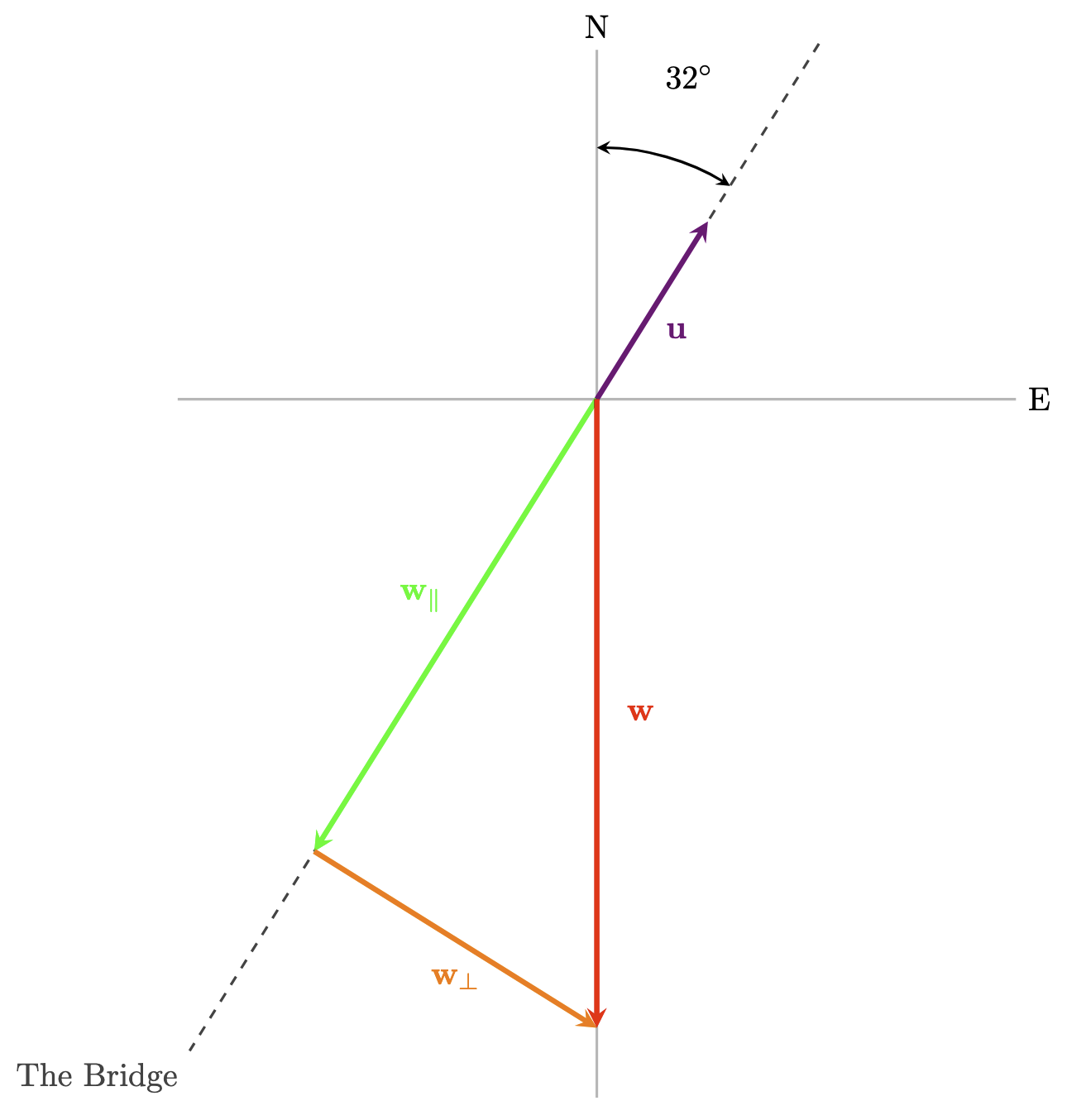
Suppose a 45 km/h wind \(\v{w}\) is blowing out of the north toward a bridge oriented \(32^\circ\) east of north. Express the corresponding wind vector as a sum of vectors, one parallel to the bridge and one perpendicular to it. Also, compute the magnitude of the perpendicular term to determine the speed of the part of the wind blowing directly at the bridge.
Hint.
Richard drew a pretty diagram based on his interpretation of this problem (by saying drawing, what he really meant is coding using TikZ...). Your goal is to find the two components of the vector \(\v{w}\text{,}\) one parallel to \(\v{u}\) and one orthogonal to \(\v{u}\text{.}\)
Figure 12.3.38. Wind vector decomposition
Solution.
We set up a coordinate system where North is the direction of the positive \(y\)-axis and East is the positive \(x\)-axis. Since the wind is blowing out of the North, it heads South, so \(\v{w} = \la 0, -45 \ra\text{.}\)
Figure 12.3.39. Wind vector decomposition
The bridge is oriented \(32^\circ\) East of North. We can define a unit vector \(\v{u}\) along the bridge direction using trigonometry: the \(x\)-component is \(\sin(58^\circ)\) and the \(y\)-component is \(\cos(58^\circ)\text{.}\)
\begin{equation*} \v{u} = \la \cos(58^\circ), \sin(58^\circ) \ra \end{equation*}
We first find \(\v{w}_\parallel\text{,}\) the vector parallel to the bridge by computing the projection of \(\v{w}\) along \(\v{u}\text{:}\)
\begin{align*} \v{w}_{\parallel} \amp= \text{proj}_{\v{u}} \v{w} = \lp \frac{\v{w} \cdot \v{u}}{\v{u} \cdot \v{u}} \rp \v{u} \\ \amp= \lp \la 0, -45 \ra \cdot \la \cos(58^\circ), \sin(58^\circ) \ra \rp \v{u} \\ \amp= -45\sin(58^\circ) \la \cos(58^\circ), \sin(58^\circ) \ra \\ \amp\approx \la -20.22, -32.36 \ra \end{align*}
Next, we find \(\v{w}_\perp\text{,}\) the vector perpendicular to the bridge by computing the difference \(\v{w}_{\perp} = \v{w} - \v{w}_{\parallel}\text{:}\)
\begin{equation*} \v{w}_{\perp} = \la 0, -45 \ra - \la -20.22, -32.36 \ra = \la 20.22, -12.64 \ra \end{equation*}
Thus, the decomposition is
\begin{equation*} \v{w} = \la -20.22, -32.36 \ra + \la 20.22, -12.64 \ra \end{equation*}
To find the speed of the wind blowing directly at the bridge, we compute the magnitude of the perpendicular component:
\begin{equation*} \|\v{w}_{\perp}\| \approx \sqrt{(20.22)^2 + (-12.64)^2} \approx 23.85 \text{ km/h} \end{equation*}

12.3.87.

Calculate the force (in newtons) required to push a 40-kg wagon up a \(10^\circ\) incline.
Figure 12.3.40.
Solution.
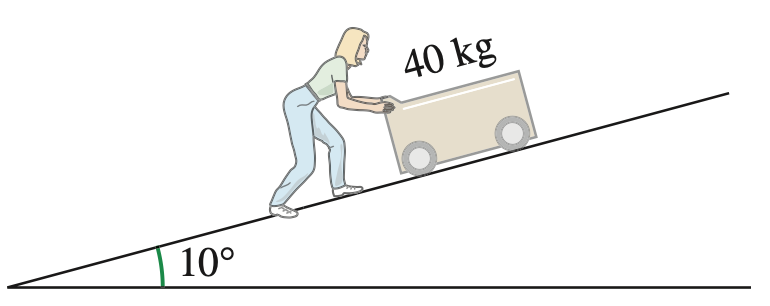
Gravity exerts a force \(\v{F}_g\) of magnitude \(40g\) newtons where \(g = 9.8\text{.}\) The magnitude of the force required to push the wagon equals the component of the force \(\v{F}_g\) along the ramp. Resolving \(\v{F}_g\) into a sum \(\v{F}_g = \v{F}_\parallel + \v{F}_\perp\text{,}\) where \(\v{F}_\parallel\) is the force along the ramp and \(\v{F}_\perp\) is the force orthogonal to the ramp, we need to find the magnitude of \(\v{F}_\parallel\text{.}\)
Figure 12.3.41.
The angle between \(\v{F}_g\) and the ramp is \(90^\circ - 10^\circ = 80^\circ\text{.}\) Hence,
\begin{equation*} \v{F}_\parallel = \|\v{F}_g\| \cos(80^\circ) = 40 \cdot 9.8 \cdot \cos(80^\circ) \approx 68.07 \text{ N} \end{equation*}
Therefore the minimum force required to push the wagon is \(68.07\) N.
Actually, this is the force required to keep the wagon from sliding down the hill; any slight amount greater than this force will serve to push it up the hill.

12.3.91.

Prove that \(\|\v{v} + \v{w}\|^2 - \|\v{v} - \v{w}\|^2 = 4\v{v} \cdot \v{w}\text{.}\)
Solution.
We expand the left-hand side using the property \(\|\v{u}\|^2 = \v{u} \cdot \v{u}\) and the distributive property of the dot product.
First, we expand the term \(\|\v{v} + \v{w}\|^2\text{:}\)
\begin{align*} \|\v{v} + \v{w}\|^2 \amp= (\v{v} + \v{w}) \cdot (\v{v} + \v{w}) \\ \amp= \v{v} \cdot \v{v} + \v{v} \cdot \v{w} + \v{w} \cdot \v{v} + \v{w} \cdot \v{w} \\ \amp= \|\v{v}\|^2 + 2(\v{v} \cdot \v{w}) + \|\v{w}\|^2 \end{align*}
Next, we expand the term \(\|\v{v} - \v{w}\|^2\text{:}\)
\begin{align*} \|\v{v} - \v{w}\|^2 \amp= (\v{v} - \v{w}) \cdot (\v{v} - \v{w}) \\ \amp= \v{v} \cdot \v{v} - \v{v} \cdot \v{w} - \v{w} \cdot \v{v} + \v{w} \cdot \v{w} \\ \amp= \|\v{v}\|^2 - 2(\v{v} \cdot \v{w}) + \|\v{w}\|^2 \end{align*}
Finally, we subtract the second expression from the first:
\begin{align*} \|\v{v} + \v{w}\|^2 - \|\v{v} - \v{w}\|^2 \amp= \lp \|\v{v}\|^2 + 2(\v{v} \cdot \v{w}) + \|\v{w}\|^2 \rp - \lp \|\v{v}\|^2 - 2(\v{v} \cdot \v{w}) + \|\v{w}\|^2 \rp \\ \amp= \|\v{v}\|^2 + 2(\v{v} \cdot \v{w}) + \|\v{w}\|^2 - \|\v{v}\|^2 + 2(\v{v} \cdot \v{w}) - \|\v{w}\|^2 \\ \amp= 4\v{v} \cdot \v{w} \end{align*}