
Section 14.5 The Gradient and Directional Derivatives

In the previous section, we learned how to calculate partial derivatives, which represent the rate of change of a function as we move strictly parallel to the \(x\)-axis or the \(y\)-axis. However, there are infinitely many other directions we can move on the surface. In this section, we will discuss how to take the derivative of a function in an arbitrary direction.
Partial derivatives tell us about the rate of change of a function at a point in the direction parallel to the \(x\)-axis and the \(y\)-axis. But there are a lot more directions we can move on the surface. How do we measure the rate of change of a function at a point in an arbitrary direction? Directional Derivative will tell us about it!

Subsection Directional Derivatives

Directional derivatives, as the name suggests, measure the rate of change of a function at a point in a specified direction. Let’s come up with the definition of directional derivatives!
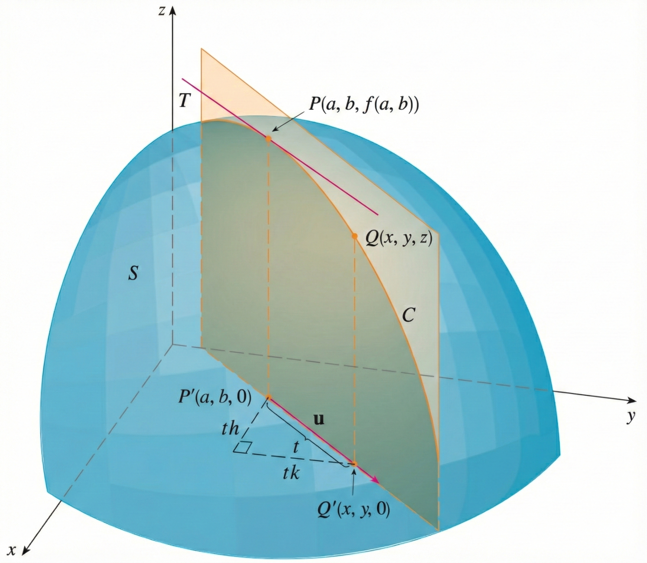
Let \(z = f(x,y)\) and \(P = (a,b,f(a,b))\) be a point on the surface. Let’s say we want to find the directional derivative of \(f\) at \(P\) in the direction of the unit vector \(\v{u} = \la h,k \ra\text{.}\) The diagram below shows this situation.
Figure 14.5.1.
The vector \(\v{u}\) and the point \(P\) can determine a vertical plane shown in the figure. This plane intersects the surface in a curve \(\c{C}\text{.}\) Then we can for sure construct a tangent line \(T\) to the curve \(\c{C}\) at the point \(P\text{.}\) Our job here is to find the slope of this tangent line.
Let’s pick another point \(Q(x,y,f(x,y))\) on the curve \(\c{C}\text{.}\) But can we express \(x\) and \(y\) in terms of a single parameter?
Yes we can! The easiest way to do so is to project \(P\) and \(Q\) onto the \(xy\)-plane, resulting in \(P' = (a,b,0)\) and \(Q' = (x,y,0)\text{,}\) respectively. Since \(\overrightarrow{P'Q'} = \la x - a, y - b \ra\) is parallel to \(\v{u}\text{,}\) then
\begin{equation*} \overrightarrow{P'Q'} = t\v{u} = t \la h,k \ra = \la th, tk \ra \end{equation*}
which implies that \(x = a + th\) and \(y = b + tk\text{.}\) Hence, we can express \(Q\) as \(Q(t) = (a + th, b + tk, f(a + th, b + tk))\) (as opposed to keeping track of two new independent variables).
Now we are ready to find the slope of the line \(T\text{!}\) Recall the slope of the line is the rise over the run. Clearly, the rise is the change in the \(z\)-coordinate and the run is the change in the distance between \(P\) and \(Q\text{,}\) which is \(t\text{.}\) Then the slope of the secant line (the line passing through \(P\) and \(Q\)) is
\begin{equation*} \frac{\Delta z}{t} = \frac{f(a + th, b + tk) - f(a,b)}{t} \end{equation*}
This implies that the slope of the tangent line \(T\) is
\begin{equation*} \lim_{t \to 0} \frac{f(a + th, b + tk) - f(a,b)}{t} \end{equation*}
This is the definition of the directional derivative!

Note 14.5.3. But Richard... How is this related to the partial derivatives?

It turns out that the directional derivative is the generalization of the partial derivatives. That is, we can recover the partial derivatives from the directional derivative by choosing the appropriate direction.
Let’s say we pick the unit vector of \(\v{i} = \la 1,0 \ra\text{.}\) Then a point \(P\) along this direction \(\v{i}\) can determine a vertical plane parallel to the \(xz\)-plane. On this plane, the \(y\)-coordinate is fixed. So we expect the directional derivative to be \(f_x\text{.}\)
Using the definition of the directional derivative, we have
\begin{align*} D_\v{i} f(a,b) \amp= \lim_{t\to 0} \frac{f(a + t(1), b + t(0)) - f(a,b)}{t} \\ \amp= \frac{f(a + t, b) - f(a,b)}{t} \\ \amp= f_x(a,b) \end{align*}
So things work out great!
Similarly, if we pick the unit vector \(\v{j} = \la 0,1 \ra\text{,}\) then the vertical plane determined by \(P\) and \(\v{j}\) is parallel to the \(yz\)-plane. On this plane, the \(x\)-coordinate is fixed. So we expect the directional derivative to be \(f_y\text{.}\)
Using the definition of the directional derivative, we have
\begin{align*} D_\v{j} f(a,b) \amp= \lim_{t\to 0} \frac{f(a + t(0), b + t(1)) - f(a,b)}{t} \\ \amp= \frac{f(a, b + t) - f(a,b)}{t} \\ \amp= f_y(a,b) \end{align*}
So things work out great again!
But no one likes to compute the directional derivative using the limit definition every time. So we want to find a more efficient formula for the directional derivative. The following theorem gives us a nice formula for the directional derivative in terms of the partial derivatives.

Proof.

The proof of this theorem isn’t too bad but it needs a clever setup. Richard will set up the proof for you and feel free to give it a try on your own!
Hint.
Let’s define a new function \(g(t) = f(a + th, b + tk)\text{.}\) Then what is \(g'(0)\) using the definition of the derivative (the one with the limit)?
Alternatively, what is \(g'(0)\) using the Chain Rule covered in SectionΒ 14.6?
Equating the two expressions for \(g'(0)\) will give us the desired formula!
Solution. The actual proof!
Let \(g(t) = f(a + th, b + tk)\text{.}\) Then using the definition of the derivative, we have
\begin{align*} g'(0) \amp= \lim_{t\to 0} \frac{g(t) - g(0)}{t} \\ \amp= \lim_{t\to 0} \frac{f(a + th, b + tk) - f(a,b)}{t} \\ \amp= D_\v{u} f(a,b) \end{align*}
We have established that \(g'(0)\) is the directional derivative of \(f\) at \(P\) in the direction of \(\v{u}\text{.}\)
Alternatively, we can rewrite \(g(t) = f(x,y)\text{,}\) where \(x = a + th\) and \(y = b + tk\text{.}\) Using the Chain Rule in SectionΒ 14.6, we have
\begin{align*} g'(t) \amp= \frac{\partial f}{\partial x} \frac{dx}{dt} + \frac{\partial f}{\partial y} \frac{dy}{dt} = f_x(x,y) h + f_y(x,y) k \end{align*}
When \(t = 0\text{,}\) this gives us
\begin{align*} g'(0) \amp= f_x(a,b) h + f_y(a,b) k \end{align*}
Putting them together, we obtain
\begin{equation*} D_\v{u} f(a,b) = g'(0) = f_x(a,b) h + f_y(a,b) k = \la f_x(a,b), f_y(a,b) \ra \cdot \la h,k \ra \end{equation*}
as desired.

Example 14.5.5.

Find the directional derivative \(D_\v{u} f(x,y)\) if \(f(x,y) = x^3 - 3xy + 4y^2\) and \(\v{u}\) is the unit vector given by the angle \(\theta = \frac{\pi}{6}\text{.}\)
What is \(D_\v{u} f(1,2)\) and what does it mean graphically?
Hint.
We are given the function \(f\) but the unit vector isn’t given explicitly.
Well there is a formula that allows to obtain the unit vector from the angle in SectionΒ 12.1. Have fun digging!
To help you visualize the situation, Richard coded the following graph for you!
Figure 14.5.6. The Graph of \(f(x,y) = x^2 - 3xy + 4y^2\)
Solution.
First, let’s find the unit vector \(\v{u}\text{.}\) Since \(\theta = \frac{\pi}{6}\text{,}\) we have
\begin{equation*} \v{u} = \la \cos\lp\frac{\pi}{6}\rp, \sin\lp\frac{\pi}{6}\rp \ra = \la \frac{\sqrt{3}}{2}, \frac{1}{2} \ra \end{equation*}
Next, we compute the partial derivatives of \(f(x,y)\text{:}\)
\begin{equation*} f_x(x,y) = 3x^2 - 3y \qquad \text{and} \qquad f_y(x,y) = -3x + 8y \end{equation*}
Now we can find the general formula for the directional derivative:
\begin{align*} D_\v{u} f(x,y) \amp= \la 3x^2 - 3y, -3x + 8y \ra \cdot \la \frac{\sqrt{3}}{2}, \frac{1}{2} \ra \\ \amp= \frac{\sqrt{3}}{2}(3x^2 - 3y) + \frac{1}{2}(-3x + 8y) \end{align*}
Finally, to find \(D_\v{u} f(1,2)\text{,}\) we substitute \(x=1\) and \(y=2\) into the partial derivatives:
\begin{equation*} f_x(1,2) = 3(1)^2 - 3(2) = 3 - 6 = -3 \end{equation*}
\begin{equation*} f_y(1,2) = -3(1) + 8(2) = -3 + 16 = 13 \end{equation*}
So, the directional derivative is:
\begin{align*} D_\v{u} f(1,2) \amp= \la -3, 13 \ra \cdot \la \frac{\sqrt{3}}{2}, \frac{1}{2} \ra \\ \amp= \frac{-3\sqrt{3} + 13}{2} \\ \amp\approx 3.9 \end{align*}
Graphically, this value represents the slope of the tangent line of the curve obtained by intersecting the surface with the vertical plane determined by the point \(P(1,2)\) and the direction of \(\v{u}\text{.}\)

Subsection The Gradient

Observing the formula for computing the directional derivative, one of the vectors consists of the first-order partial derivatives of the function. This vector is called the gradient of the function.

Definition 14.5.7.

The gradient of a function \(f(x,y)\) at a point \(P = (a,b)\) is the vector
\begin{equation*} \nabla f(a,b) = \la f_x(a,b), f_y(a,b) \ra \end{equation*}
In three variables, for \(f(x,y,z)\) and \(P = (a,b,c)\text{,}\) the gradient is
\begin{equation*} \nabla f(a,b,c) = \la f_x(a,b,c), f_y(a,b,c), f_z(a,b,c) \ra \end{equation*}
Sometimes the notation can be a bit sloppy and we might drop the reference to the point \(P\) and just write \(\nabla f = \la \dfrac{\partial f}{\partial x}, \dfrac{\partial f}{\partial y} \ra\text{.}\) Or maybe the reference to the point becomes a subscript and we write \(\nabla f_P\text{.}\) They all mean the same thing.
The symbol to denote the gradient, \(\nabla\text{,}\) is called "del". This is an upside-down Delta. The concept of gradient can be extended to functions of \(n\) variables. We will just need to take all the first-order partial derivatives and organize them into a vector. That is, the gradient of \(f(x_1, x_2, \dots, x_n)\) is
\begin{equation*} \nabla f = \la \frac{\partial f}{\partial x_1}, \frac{\partial f}{\partial x_2}, \dots, \frac{\partial f}{\partial x_n} \ra \end{equation*}
Likewise, if we are dealing with functions of a single variable, then the gradient is just the derivative of the function. You can think of the gradient of functions of a single variable, aka the derivative, as a vector if you want but there are only two directions to move on the curve: forward (positive) and backward (negative).

Example 14.5.8.

Find the gradient of the function \(f(x,y) = \sin(3x + 2y)\) at the point \(\lp \pi, \dfrac{3\pi}{2} \rp\text{.}\)
Solution.
To find the gradient of the function \(f(x,y)\text{,}\) we first calculate the partial derivatives with respect to \(x\) and \(y\text{.}\)
Using the chain rule, the partial derivative with respect to \(x\) is:
\begin{equation*} f_x(x,y) = \frac{\partial}{\partial x} \sin(3x + 2y) = 3\cos(3x + 2y) \end{equation*}
The partial derivative with respect to \(y\) is:
\begin{equation*} f_y(x,y) = \frac{\partial}{\partial y} \sin(3x + 2y) = 2\cos(3x + 2y) \end{equation*}
Now we evaluate these partial derivatives at the point \(\lp \pi, \dfrac{3\pi}{2} \rp\text{.}\) First, we determine the value inside the cosine function:
\begin{equation*} 3(\pi) + 2\lp \dfrac{3\pi}{2} \rp = 3\pi + 3\pi = 6\pi \end{equation*}
Since \(\cos(6\pi) = 1\text{,}\) we have:
\begin{align*} f_x\lp \pi, \dfrac{3\pi}{2} \rp \amp = 3(1) = 3\\ f_y\lp \pi, \dfrac{3\pi}{2} \rp \amp = 2(1) = 2 \end{align*}
Thus, the gradient vector is:
\begin{equation*} \nabla f\lp \pi, \dfrac{3\pi}{2} \rp = \langle 3, 2 \rangle \end{equation*}
There are some nice properties of the gradient. The proofs should be super straightforward (just use the properties of derivative plus vectors to push the symbols around). So Richard will just state the properties without proof.
Remember we picked out the gradient from the formula for computing the directional derivative, so we can rewrite the formula for computing the directional derivative as
\begin{equation*} D_\v{u} f(P) = \nabla f_P \cdot \v{u} \end{equation*}
But what is the difference between the gradient and the directional derivative, as they both seem to be related to the rate of change of the function at a point?
The short answer is that the gradient is a vector while the directional derivative is a scalar. We can actually learn more about the relationship between them from this formula.
Notice that the directional derivative is the dot product of the gradient and the unit vector. A property of the dot product tells us that
\begin{equation*} D_\v{u} f(P) = \|\nabla f_P\| \|u\| \cos(\theta) = \|\nabla f_P\| \cos(\theta) \end{equation*}
where \(\theta\) is the angle between the gradient and the unit vector. That is, the directional derivative (aka the rate of change of the function at a point in a specific direction) varies with the cosine of the angle \(\theta\) between the gradient and the direction. Since \(\cos(\theta)\) is bounded by \(-1\) and \(1\text{,}\) then we have
\begin{equation*} - \|\nabla f_P\| \leq D_\v{u} f(P) \leq \|\nabla f_P\| \end{equation*}
Observe that \(D_\v{u} f(P) = \|\nabla f_P\|\) when \(\theta = 0\) (i.e., when \(\v{u}\) is in the same direction of \(\nabla f_P\)). That is, the gradient points in the direction of the maximum rate of increase, and this maximum rate is \(\|\nabla f_P\|\). Let’s make it into a cool theorem!
We haven’t talked about the last part of the theorem yet, so let’s focus on the first two parts for now.

Example 14.5.11.

Let \(f(x,y) = xe^y\text{.}\)
  1. Find the rate of change of \(f\) at the point \(P(2,0)\) in the direction from \(P\) to \(Q\lp \frac{1}{2}, \frac{1}{2} \rp\text{.}\)
  2. In what direction does \(f\) have the maximum rate of increase at \(P\text{?}\) What is this maximum rate of increase?
Solution.
First, we calculate the gradient of \(f(x,y) = xe^y\text{:}\)
\begin{equation*} \nabla f(x,y) = \la e^y, xe^y \ra \end{equation*}
At the point \(P(2,0)\text{,}\) the gradient vector is:
\begin{equation*} \nabla f(2,0) = \la e^0, 2(e^0) \ra = \la 1, 2 \ra \end{equation*}
  1. We find the vector representing the direction from \(P\) to \(Q\text{:}\)
    \begin{equation*} \overrightarrow{PQ} = \la \frac{1}{2} - 2, \frac{1}{2} - 0 \ra = \la -\frac{3}{2}, \frac{1}{2} \ra \end{equation*}
    Next, we find the unit vector \(\mathbf{u}\) in this direction:
    \begin{equation*} |\overrightarrow{PQ}| = \sqrt{\lp -\frac{3}{2} \rp^2 + \lp \frac{1}{2} \rp^2} = \sqrt{\frac{10}{4}} = \frac{\sqrt{10}}{2} \end{equation*}
    \begin{equation*} \mathbf{u} = \frac{\vec{PQ}}{|\vec{PQ}|} = \la -\frac{3}{\sqrt{10}}, \frac{1}{\sqrt{10}} \ra \end{equation*}
    The rate of change is the directional derivative \(D_{\mathbf{u}}f(2,0)\text{:}\)
    \begin{align*} D_{\mathbf{u}}f(2,0) = \nabla f(2,0) \cdot \mathbf{u} \amp = \la 1, 2 \ra \cdot \la -\frac{3}{\sqrt{10}}, \frac{1}{\sqrt{10}} \ra\\ \amp = -\frac{3}{\sqrt{10}} + \frac{2}{\sqrt{10}}\\ \amp = -\frac{1}{\sqrt{10}} \end{align*}
  2. The function has the maximum rate of increase in the direction of the gradient vector:
    \begin{equation*} \la 1, 2 \ra \end{equation*}
    The maximum rate of increase is the magnitude of the gradient:
    \begin{equation*} |\nabla f(2,0)| = \sqrt{1^2 + 2^2} = \sqrt{5} \end{equation*}
Now that we know the difference between the gradient and the directional derivative, we will debrief the last part of the theorem that says the gradient is always normal to the level curve (or surface) at the point.
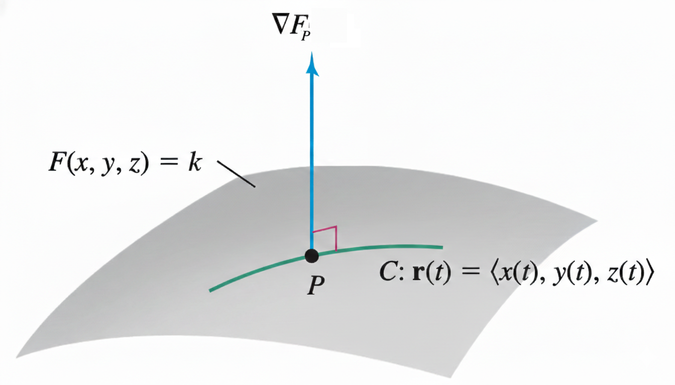
Let’s say we have a surface \(S\) in \(\R^3\text{.}\) Then we will need an equation of three variables to describe the surface. That is, the surface will have an equation \(F(x,y,z) = k\) (this also means that the surface is a level surface of the function \(f\)).
Now imagine there is a point \(P\) on the surface and a curve \(\v{C}\) on the surface passing through \(P = (a,b,c)\text{.}\) If we call the curve \(\v{r}(t) = \la x(t), y(t), z(t) \ra\text{,}\) then there is a parameter \(t_0\) such that \(\v{r}(t_0) = \la a,b,c \ra\text{.}\) Since \(\c{C}\) lies on the surface, then we obtain
\begin{equation*} F\lp \v{r}(t) \rp = F\lp x(t), y(t), z(t) \rp = k \end{equation*}
If everything is nice and differentiable, then we can differentiate both sides of the equation using the Chain Rule in SectionΒ 14.6 to get
\begin{align*} \frac{\partial F}{\partial x} \frac{dx}{dt} + \frac{\partial F}{\partial y} \frac{dy}{dt} + \frac{\partial F}{\partial z} \frac{dz}{dt} \amp= 0 \\ \la \frac{\partial F}{\partial x}, \frac{\partial F}{\partial y}, \frac{\partial F}{\partial z} \ra \cdot \la \frac{dx}{dt}, \frac{dy}{dt}, \frac{dz}{dt} \ra \amp= 0 \\ \nabla f_P \cdot \v{r}'(t_0) \amp= 0 \end{align*}
The diagram below shows the situation.
Figure 14.5.12.
We basically just showed that the gradient vectors are normal to the surface!
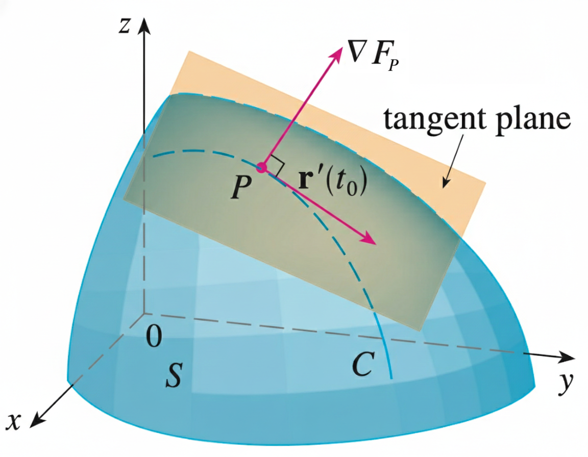
Hmm but why do we need a normal vector to the surface at a point? We can find an equation of the tangent plane using the gradient vector and the point! If you compare the formula for the tangent plane in SectionΒ 14.4, the normal vector is exactly the gradient vector!
Figure 14.5.14.
Using this theorem, we can find an equation of the tangent plane to a surface without needing an explicit formula for our function. That is, \(z\) doesn’t need to be isolated in the equation of the surface.

Example 14.5.15.

Find the equation of the tangent plane at the point \(P = (-2,1,-3)\) to the ellipsoid
\begin{equation*} \frac{x^2}{4} + y^2 + \frac{z^2}{9} = 3 \end{equation*}
Solution.
Let \(F(x,y,z) = \frac{x^2}{4} + y^2 + \frac{z^2}{9}\text{.}\) Then the ellipsoid is the level surface \(F(x,y,z) = 3\text{.}\) +We find the gradient vector to determine the normal vector to the surface.
\begin{equation*} \nabla F(x,y,z) = \la \frac{x}{2}, 2y, \frac{2z}{9} \ra \end{equation*}
Evaluate the gradient at the point \(P(-2,1,-3)\) to find the normal vector \(\v{n}\text{:}\)
\begin{equation*} \mathbf{n} = \nabla F(-2,1,-3) = \la -1, 2, -\frac{2}{3} \ra \end{equation*}
The equation of the tangent plane at \(P\) is:
\begin{align*} -1(x - (-2)) + 2(y - 1) - \frac{2}{3}(z - (-3)) \amp = 0\\ -(x + 2) + 2(y - 1) - \frac{2}{3}(z + 3) \amp = 0 \end{align*}
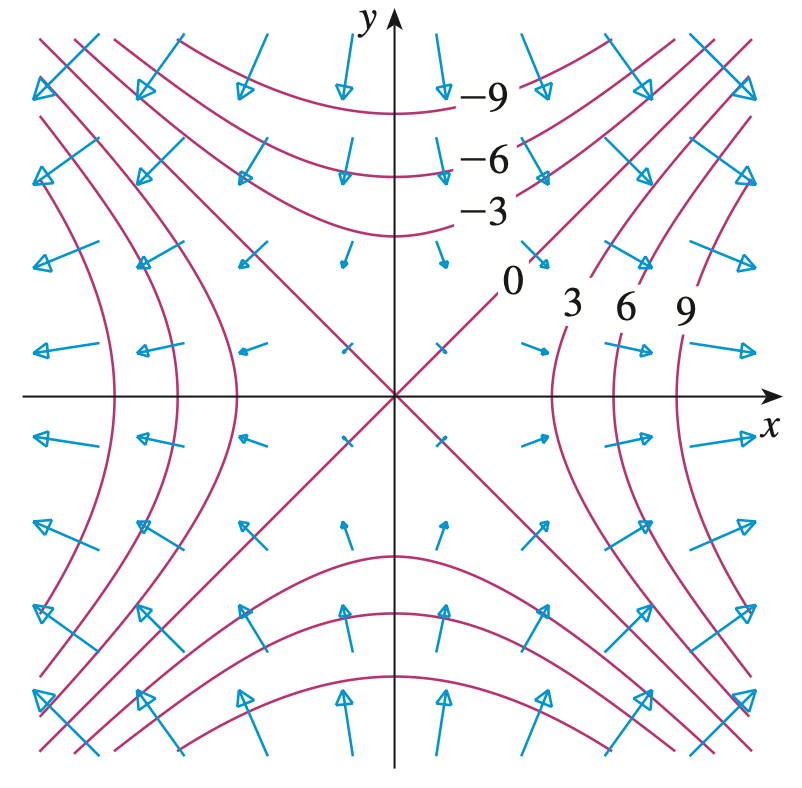
Now that we know what the gradient is (pointing in the direction of the maximum rate of increase) and how it behaves (normal to the level curve/surface), we can create something called the gradient vector field (which is super similar to the vector field you learned back in MTH 253). For example, the gradient vector field of \(f(x,y) = x^2 - y^2\text{,}\) superimposed on a contour map, is shown below.
Figure 14.5.16.
As expected, the gradient vectors are normal to the level curves. They also point in the direction of the maximum rate of increase. That is, each gradient vector is pointing "uphill".
Below is the graph of the function \(f(x,y) = x^2 - y^2\text{.}\) Try to convince yourself that the gradient vectors are indeed pointing in the direction of the maximum rate of increase and that they are normal to the level curves.
Figure 14.5.17. The surface \(f(x,y) = x^2 - y^2\)
Gradient is an important concept that helps us understand the behavior of the surface. We will see more applications of the gradient in the following sections when we talk about optimization. Just a quick preview: if all the gradient vectors are pointing toward the same point on the gradient vector field, then that point is a local maximum since the surface is going uphill towards this point.

Worksheet Assigned Problems for Section 14.5

The problems listed below are assigned to be included in your problem set portfolio. Note that a specific selection of these problems will also form the written homework assignments. I recommend working through all of them to ensure a solid grasp of the material. Reach out to Richard for help if you get stuck or have any questions.
The solutions will be posted after the written homework due dates. If you have any questions about your work, talk to Richard and he is happy to discuss the process with you.

14.5.5.

Calculate the gradient of \(f(x,y) = \cos\lp x^2 + y \rp\text{.}\)
Solution.
To find the gradient \(\nabla f(x,y)\text{,}\) we compute the partial derivatives with respect to \(x\) and \(y\) using the Chain Rule.
Partial derivative with respect to \(x\text{:}\)
\begin{equation*} f_x(x,y) = \frac{\partial}{\partial x} \cos(x^2 + y) = -\sin(x^2 + y) \cdot \frac{\partial}{\partial x}(x^2 + y) = -2x\sin(x^2 + y) \end{equation*}
Partial derivative with respect to \(y\text{:}\)
\begin{equation*} f_y(x,y) = \frac{\partial}{\partial y} \cos(x^2 + y) = -\sin(x^2 + y) \cdot \frac{\partial}{\partial y}(x^2 + y) = -\sin(x^2 + y) \end{equation*}
Thus, the gradient vector is:
\begin{equation*} \nabla f(x,y) = \la -2x\sin(x^2 + y), -\sin(x^2 + y) \ra \end{equation*}

14.5.17.

Use the Chain Rule to calculate \(\dfrac{d}{dt} f(\v{r}(t))\text{,}\) where
\begin{equation*} f(x,y) = \ln(x) + \ln(y) \qquad \text{ and } \qquad \v{r}(t) = \la \cos(t), t^2 \ra \end{equation*}
at the point where \(t = \dfrac{\pi}{4}\text{.}\)
Solution.
According to the Chain Rule for paths, \(\frac{d}{dt} f(\v{r}(t)) = \nabla f(\v{r}(t)) \cdot \v{r}'(t)\text{.}\)
First, let’s find the gradient of \(f\text{:}\)
\begin{equation*} \nabla f(x,y) = \la \frac{\partial}{\partial x}(\ln x + \ln y), \frac{\partial}{\partial y}(\ln x + \ln y) \ra = \la \frac{1}{x}, \frac{1}{y} \ra \end{equation*}
Next, let’s find the derivative of the path \(\v{r}(t)\text{:}\)
\begin{equation*} \v{r}'(t) = \la \frac{d}{dt}\cos(t), \frac{d}{dt}t^2 \ra = \la -\sin(t), 2t \ra \end{equation*}
Now we evaluate both at \(t = \frac{\pi}{4}\text{.}\)
\begin{equation*} \v{r}\lp \frac{\pi}{4} \rp = \la \cos\lp \frac{\pi}{4} \rp, \lp \frac{\pi}{4} \rp^2 \ra = \la \frac{\sqrt{2}}{2}, \frac{\pi^2}{16} \ra \end{equation*}
So at this point, \(x = \frac{\sqrt{2}}{2}\) and \(y = \frac{\pi^2}{16}\text{.}\)
\begin{equation*} \nabla f\lp \v{r}\lp \frac{\pi}{4} \rp \rp = \la \frac{1}{\sqrt{2}/2}, \frac{1}{\pi^2/16} \ra = \la \sqrt{2}, \frac{16}{\pi^2} \ra \end{equation*}
And the velocity vector is:
\begin{equation*} \v{r}'\lp \frac{\pi}{4} \rp = \la -\sin\lp \frac{\pi}{4} \rp, 2\lp \frac{\pi}{4} \rp \ra = \la -\frac{\sqrt{2}}{2}, \frac{\pi}{2} \ra \end{equation*}
Finally, compute the dot product:
\begin{align*} \frac{d}{dt} f\lp \v{r}\lp \frac{\pi}{4} \rp \rp \amp= \la \sqrt{2}, \frac{16}{\pi^2} \ra \cdot \la -\frac{\sqrt{2}}{2}, \frac{\pi}{2} \ra \\ \amp= (\sqrt{2})\lp -\frac{\sqrt{2}}{2} \rp + \lp \frac{16}{\pi^2} \rp \lp \frac{\pi}{2} \rp \\ \amp= -1 + \frac{8}{\pi} \end{align*}

14.5.25.

Calculate the directional derivative of \(f(x,y) = \tan^{-1}(xy)\) in the direction of \(\v{v} = \la 1,1 \ra\) at the point \(P = (3,4)\text{.}\) Remember to use a unit vector in your directional derivative computation.
Solution.
First, find the gradient \(\nabla f(x,y)\text{:}\)
\begin{align*} f_x(x,y) \amp= \frac{1}{1+(xy)^2} \cdot y = \frac{y}{1+x^2y^2} \\ f_y(x,y) \amp= \frac{1}{1+(xy)^2} \cdot x = \frac{x}{1+x^2y^2} \end{align*}
Evaluate the gradient at \(P(3,4)\text{:}\)
\begin{align*} f_x(3,4) \amp= \frac{4}{1+(3^2)(4^2)} = \frac{4}{1+144} = \frac{4}{145} \\ f_y(3,4) \amp= \frac{3}{1+(3^2)(4^2)} = \frac{3}{1+144} = \frac{3}{145} \\ \nabla f(3,4) \amp= \la \frac{4}{145}, \frac{3}{145} \ra \end{align*}
Next, find the unit vector \(\v{u}\) in the direction of \(\v{v} = \la 1,1 \ra\text{:}\)
\begin{align*} \|\v{v}\| \amp= \sqrt{1^2 + 1^2} = \sqrt{2} \\ \v{u} \amp= \frac{\v{v}}{\|\v{v}\|} = \la \frac{1}{\sqrt{2}}, \frac{1}{\sqrt{2}} \ra \end{align*}
Finally, calculate the directional derivative using the dot product:
\begin{align*} D_\v{u}f(3,4) \amp= \nabla f(3,4) \cdot \v{u} \\ \amp= \la \frac{4}{145}, \frac{3}{145} \ra \cdot \la \frac{1}{\sqrt{2}}, \frac{1}{\sqrt{2}} \ra \\ \amp= \frac{4}{145\sqrt{2}} + \frac{3}{145\sqrt{2}} \\ \amp= \frac{7}{145\sqrt{2}} = \frac{7\sqrt{2}}{290} \end{align*}

14.5.35.

Determine the direction in which \(f(x,y,z) = \dfrac{xy}{z}\) has maximum rate of increase from \(P = (1,-1,3)\text{,}\) and give the rate of change in that direction.
Solution.
The direction of maximum increase is given by the gradient \(\nabla f(P)\text{,}\) and the rate is the magnitude \(\|\nabla f(P)\|\text{.}\)
First, calculate the partial derivatives:
\begin{align*} f_x \amp= \frac{y}{z} \\ f_y \amp= \frac{x}{z} \\ f_z \amp= -\frac{xy}{z^2} \end{align*}
Evaluate at \(P(1,-1,3)\text{:}\)
\begin{align*} f_x(1,-1,3) \amp= \frac{-1}{3} = -\frac{1}{3} \\ f_y(1,-1,3) \amp= \frac{1}{3} \\ f_z(1,-1,3) \amp= -\frac{(1)(-1)}{3^2} = \frac{1}{9} \end{align*}
So the direction of maximum increase is:
\begin{equation*} \nabla f(1,-1,3) = \la -\frac{1}{3}, \frac{1}{3}, \frac{1}{9} \ra \end{equation*}
The maximum rate of change is the magnitude:
\begin{align*} \|\nabla f\| \amp= \sqrt{\lp -\frac{1}{3} \rp^2 + \lp \frac{1}{3} \rp^2 + \lp \frac{1}{9} \rp^2} \\ \amp= \sqrt{\frac{1}{9} + \frac{1}{9} + \frac{1}{81}} \\ \amp= \sqrt{\frac{9}{81} + \frac{9}{81} + \frac{1}{81}} \\ \amp= \sqrt{\frac{19}{81}} = \frac{\sqrt{19}}{9} \end{align*}

14.5.37.

Suppose that \(\nabla f_P = \la 2,-4,4 \ra\text{.}\) Is \(f\) increasing or decreasing at \(P\) in the direction of \(\v{v} = \la 2,1,3 \ra\text{?}\)
Solution.
To determine if \(f\) is increasing or decreasing, we check the sign of the directional derivative \(D_\v{u}f(P)\text{.}\) The sign of \(D_\v{u}f\) is the same as the sign of the dot product \(\nabla f_P \cdot \v{v}\) (since dividing by \(\|\v{v}\|\) to get \(\v{u}\) is always positive).
Calculate the dot product:
\begin{align*} \nabla f_P \cdot \v{v} \amp= \la 2, -4, 4 \ra \cdot \la 2, 1, 3 \ra \\ \amp= (2)(2) + (-4)(1) + (4)(3) \\ \amp= 4 - 4 + 12 = 12 \end{align*}
Since the dot product is positive (\(12 > 0\)), the directional derivative is positive. Therefore, \(f\) is increasing in the direction of \(\v{v}\text{.}\)

14.5.39.

Let \(f(x,y,z) = \sin(xy + z)\) and \(P = (0,-1, \pi)\text{.}\) Calculate \(D_\v{u} f(P)\text{,}\) where \(\v{u}\) is a unit vector making an angle \(\theta = 30^\circ\) with \(\nabla f_P\text{.}\)
Solution.
We use the formula \(D_\v{u} f(P) = \|\nabla f_P\| \cos(\theta)\text{.}\)
First, compute the gradient \(\nabla f\text{:}\)
\begin{align*} f_x \amp= y\cos(xy+z) \\ f_y \amp= x\cos(xy+z) \\ f_z \amp= \cos(xy+z) \end{align*}
Evaluate at \(P(0,-1,\pi)\text{:}\)
\begin{equation*} \text{Argument } = (0)(-1) + \pi = \pi \end{equation*}
\begin{align*} f_x(0,-1,\pi) \amp= -1\cos(\pi) = (-1)(-1) = 1 \\ f_y(0,-1,\pi) \amp= 0\cos(\pi) = 0 \\ f_z(0,-1,\pi) \amp= \cos(\pi) = -1 \end{align*}
So \(\nabla f_P = \la 1, 0, -1 \ra\text{.}\)
Next, find the magnitude of the gradient:
\begin{equation*} \|\nabla f_P\| = \sqrt{1^2 + 0^2 + (-1)^2} = \sqrt{2} \end{equation*}
Finally, calculate the directional derivative using \(\theta = 30^\circ\text{:}\)
\begin{align*} D_\v{u} f(P) \amp= \|\nabla f_P\| \cos(30^\circ) \\ \amp= \sqrt{2} \cdot \frac{\sqrt{3}}{2} = \frac{\sqrt{6}}{2} \end{align*}

14.5.43.

Find the two points on the ellipsoid
\begin{equation*} \frac{x^2}{4} + \frac{y^2}{9} + z^2 = 1 \end{equation*}
where the tangent plane is normal to \(\v{v} = \la 1,1,-2 \ra\text{.}\)
Solution.
Let \(F(x,y,z) = \frac{x^2}{4} + \frac{y^2}{9} + z^2\text{.}\) The normal vector to the tangent plane is given by the gradient \(\nabla F\text{.}\)
\begin{equation*} \nabla F = \la \frac{x}{2}, \frac{2y}{9}, 2z \ra \end{equation*}
We want the tangent plane to be normal to \(\v{v} = \la 1,1,-2 \ra\text{,}\) which means the gradient must be parallel to \(\v{v}\text{.}\) So, \(\nabla F = k \v{v}\) for some scalar constant \(k\text{.}\)
\begin{equation*} \la \frac{x}{2}, \frac{2y}{9}, 2z \ra = k \la 1, 1, -2 \ra = \la k, k, -2k \ra \end{equation*}
Equating components gives us expressions for \(x, y, z\) in terms of \(k\text{:}\)
\begin{gather*} \frac{x}{2} = k \implies x = 2k \\ \frac{2y}{9} = k \implies y = \frac{9k}{2} \\ 2z = -2k \implies z = -k \end{gather*}
Since the points must lie on the ellipsoid, substitute these into the ellipsoid equation:
\begin{align*} \frac{(2k)^2}{4} + \frac{(9k/2)^2}{9} + (-k)^2 \amp= 1 \\ \frac{4k^2}{4} + \frac{81k^2/4}{9} + k^2 \amp= 1 \\ k^2 + \frac{9k^2}{4} + k^2 \amp= 1 \\ 2k^2 + \frac{9k^2}{4} \amp= 1 \\ \frac{8k^2 + 9k^2}{4} \amp= 1 \\ \frac{17k^2}{4} \amp= 1 \implies k^2 = \frac{4}{17} \implies k = \pm \frac{2}{\sqrt{17}} \end{align*}
Now find the two points by plugging \(k\) back into our expressions for \(x,y,z\text{:}\) Case 1: \(k = \frac{2}{\sqrt{17}}\)
\begin{equation*} P_1 = \lp 2\lp\frac{2}{\sqrt{17}}\rp, \frac{9}{2}\lp\frac{2}{\sqrt{17}}\rp, -\frac{2}{\sqrt{17}} \rp = \lp \frac{4}{\sqrt{17}}, \frac{9}{\sqrt{17}}, -\frac{2}{\sqrt{17}} \rp \end{equation*}
Case 2: \(k = -\frac{2}{\sqrt{17}}\)
\begin{equation*} P_2 = \lp -\frac{4}{\sqrt{17}}, -\frac{9}{\sqrt{17}}, \frac{2}{\sqrt{17}} \rp \end{equation*}

14.5.47.

Find an equation of the tangent plane to the surface
\begin{equation*} xz + 2x^2y + y^2z^3 = 11 \end{equation*}
at the point \(P = (2,1,1)\text{.}\)
Solution.
Let \(F(x,y,z) = xz + 2x^2y + y^2z^3\text{.}\) The surface is the level set \(F=11\text{.}\) First, find the gradient \(\nabla F\text{:}\)
\begin{align*} F_x \amp= z + 4xy \\ F_y \amp= 2x^2 + 2yz^3 \\ F_z \amp= x + 3y^2z^2 \end{align*}
Evaluate at \(P(2,1,1)\) to find the normal vector:
\begin{align*} F_x(2,1,1) \amp= 1 + 4(2)(1) = 9 \\ F_y(2,1,1) \amp= 2(2)^2 + 2(1)(1)^3 = 8 + 2 = 10 \\ F_z(2,1,1) \amp= 2 + 3(1)^2(1)^2 = 2 + 3 = 5 \end{align*}
The normal vector is \(\v{n} = \la 9, 10, 5 \ra\text{.}\)
The equation of the tangent plane is:
\begin{align*} 9(x - 2) + 10(y - 1) + 5(z - 1) \amp= 0 \\ 9x - 18 + 10y - 10 + 5z - 5 \amp= 0 \\ 9x + 10y + 5z \amp= 33 \end{align*}

14.5.53.

Find a function \(f(x,y,z)\) such that \(\nabla f = \la 2x,1,2 \ra\text{.}\)
Solution.
We are given \(f_x = 2x\text{,}\) \(f_y = 1\text{,}\) and \(f_z = 2\text{.}\) We integrate each partial derivative to reconstruct \(f\text{.}\)
Integrate \(f_x\) with respect to \(x\text{:}\)
\begin{equation*} f(x,y,z) = \int 2x \, dx = x^2 + C_1(y,z) \end{equation*}
Differentiate this result with respect to \(y\) and compare to the given \(f_y\text{:}\)
\begin{equation*} \frac{\partial}{\partial y}(x^2 + C_1(y,z)) = \frac{\partial C_1}{\partial y} = 1 \end{equation*}
Integrating \(1\) with respect to \(y\) gives \(C_1(y,z) = y + C_2(z)\text{.}\) So far, \(f(x,y,z) = x^2 + y + C_2(z)\text{.}\)
Differentiate this with respect to \(z\) and compare to the given \(f_z\text{:}\)
\begin{equation*} \frac{\partial}{\partial z}(x^2 + y + C_2(z)) = C_2'(z) = 2 \end{equation*}
Integrating \(2\) with respect to \(z\) gives \(C_2(z) = 2z + K\) (where \(K\) is a constant).
Thus, a possible function is:
\begin{equation*} f(x,y,z) = x^2 + y + 2z \end{equation*}
(Any constant \(K\) can be added, but usually \(K=0\) is sufficient for "Find a function" problems).

14.5.65.

Let \(\c{C}\) be the curve of intersection of the spheres
\begin{equation*} x^3 + 2xy + yz = 7 \qquad \text{ and } \qquad 3x^2 - yz = 1 \end{equation*}
Find the parametric equations of the tangent line to \(\c{C}\) at \(P = (1,2,1)\text{.}\)
Solution.
The curve \(\c{C}\) is the intersection of two surfaces. The tangent line to \(\c{C}\) must be tangent to both surfaces. This means the direction vector of the tangent line, \(\v{v}\text{,}\) must be perpendicular to the normal vectors of both surfaces.
Let \(F(x,y,z) = x^3 + 2xy + yz\) and \(G(x,y,z) = 3x^2 - yz\text{.}\) First, find the gradients (normal vectors) at \(P(1,2,1)\text{.}\)
Gradient of \(F\text{:}\)
\begin{equation*} \nabla F = \la 3x^2 + 2y, 2x + z, y \ra \end{equation*}
At \(P(1,2,1)\text{:}\)
\begin{equation*} \nabla F(1,2,1) = \la 3(1)^2 + 2(2), 2(1) + 1, 2 \ra = \la 7, 3, 2 \ra \end{equation*}
Gradient of \(G\text{:}\)
\begin{equation*} \nabla G = \la 6x, -z, -y \ra \end{equation*}
At \(P(1,2,1)\text{:}\)
\begin{equation*} \nabla G(1,2,1) = \la 6(1), -1, -2 \ra = \la 6, -1, -2 \ra \end{equation*}
The direction vector \(\v{v}\) is the cross product of these two gradients:
\begin{align*} \v{v} \amp= \nabla F \times \nabla G \\ \amp= \begin{vmatrix} \v{i} \amp \v{j} \amp \v{k} \\ 7 \amp 3 \amp 2 \\ 6 \amp -1 \amp -2 \end{vmatrix} \\ \amp= \la (3)(-2) - (2)(-1), -((7)(-2) - (2)(6)), (7)(-1) - (3)(6) \ra \\ \amp= \la -6 + 2, -(-14 - 12), -7 - 18 \ra \\ \amp= \la -4, 26, -25 \ra \end{align*}
The tangent line passes through \(P(1,2,1)\) with direction \(\la -4, 26, -25 \ra\text{.}\) The parametric equations are:
\begin{align*} x(t) \amp= 1 - 4t \\ y(t) \amp= 2 + 26t \\ z(t) \amp= 1 - 25t \end{align*}