In single-variable Calculus (MTH 251Z or MTH 251), the derivative \(f'(x)\) gave us a powerful tool to measure the instantaneous rate of change. Geometrically, it represented the slope of the tangent line to the curve \(y=f(x)\text{.}\) Now that we are dealing with functions of two variables \(z=f(x,y)\text{,}\) the concept of "rate of change" becomes a bit more complex.
Imagine standing on the side of a mountain (a surface). The steepness of the terrain depends entirely on which direction you choose to walk! To manage this complexity, we start by restricting our movement to the coordinate directions: parallel to the \(x\)-axis or parallel to the \(y\)-axis. This approach leads us to the concept of partial derivatives. Essentially, we will look at how the function changes if we only wiggle one variable while holding the others constant.
Let \(f(x,y)\) be a function of two variables. The partial derivative of \(f\) with respect to \(x\) at the point \((a,b)\text{,}\) denoted \(f_x(a,b)\) or \(\dfrac{\partial f}{\partial x}\bigg|_{(a,b)}\text{,}\) is defined as
The partial derivative of \(f\) with respect to \(y\) at the point \((a,b)\text{,}\) denoted \(f_y(a,b)\) or \(\dfrac{\partial f}{\partial y}\bigg|_{(a,b)}\text{,}\) is defined as
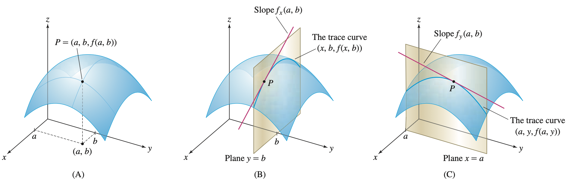
We can observe from the definition that we fix one variable and let the other variable vary to compute the partial derivative. By fixing one variable, we are essentially looking at the trace curve of the surface obtained by intersecting with a plane. Then the partial derivative is the slope of the tangent line to the trace curve at the point of interest.
You can imagine that the reason why we call them the partial derivatives is because they only measure the rate of change with respect to one variable while keeping the other variable fixed. There is a concept called the total derivative (or total differential) that takes into account the rate of change with respect to both variables. We will investigate this concept in the next section.
Symbolically, we use the symbol "\(\partial\)" to emphasize this "partial" nature. When we see "\(\frac{\partial f}{\partial x}\)", we know that that \(x\) is just one of the several variables affecting \(f\text{,}\) and the others are being held fixed. As a comparison, when we see \(\frac{df}{dx}\text{,}\) we know that \(x\) is the only variable affecting \(f\text{.}\)
If this were a MTH 251Z (or MTH 251), then Richard would make you to evaluate the limits using the definition to get a sense of what the derivative measures (the limit of some average rate of change as the change gets smaller and smaller). However, this is MTH 254 so Richard assumes you are already comfortable with this concept. Feel free to use the derivative formulas and rules that you learned from MTH 251Z (or MTH 251) to compute partial derivatives.
Compute \(\dfrac{\partial f}{\partial x}\) at the point \((2,-4)\text{.}\) Also, interpret the meaning of this value in terms of the graph of \(f\text{.}\)
Compute \(\dfrac{\partial f}{\partial y}\) at the point \((2,-4)\text{.}\) Also, interpret the meaning of this value in terms of the graph of \(f\text{.}\)
If you stare at the definition of the partial derivative, we either treat \(x\) or \(y\) as the variable and the other as a constant. This will help you to evaluate the partial derivatives using the rules you already know!
This means that the slope of the tangent line to the trace of the surface obtained by intersecting with the plane \(y=-4\) at the point \((2,-4,6)\) is 12.
This means that the slope of the tangent line to the trace of the surface obtained by intersecting with the plane \(x=2\) at the point \((2,-4,6)\) is 8.
We can find the higher order partial derivatives by taking the partial derivatives of the partial derivatives. Since we have two variables, we can take the partial derivatives in different orders.
Observe that the two mixed partial derivatives \(f_{xy}\) and \(f_{yx}\) are the same in this example. It turns out that most of the functions we encounter have this property. A French mathematician Alexis Clairaut (1713-1765) also found this pattern, formulate it as a theorem, and proved it.
If \(f_{xy}\) and \(f_{yx}\) both exist and are continuous on a disk \(D\text{,}\) then \(f_{xy}(a,b) = f_{yx}(a,b)\) for all points \((a,b) \in D\text{.}\) Therefore, on \(D\text{,}\)
\begin{equation*}
\frac{\partial^2 f}{\partial x \partial y} = \frac{\partial^2 f}{\partial y \partial x}
\end{equation*}
The proof of Clairaut’s Theorem is a bit technical and requires the Mean Value Theorem. If you are interested in seeing the proof, you can check out the textbook on page A21.
The Clairaut’s Theorem states that if the mixed partial derivatives are continuous, then the order of differentiation does not matter. This result can be generalized to higher order partial derivatives as well. That is, we can interchange the order of differentiation as long as the mixed partial derivatives are continuous.
Clairaut’s Theorem allows us to rearrange the order of differentiation as long as the mixed partial derivatives are continuous. So which order of differentiation would be the easiest to compute?
From here, we can conclude that the rest of the derivatives will also be zero since we are taking the derivative of a constant. Therefore, \(f_{uvxyvu} = f_{vxuyvu} = 0\text{.}\)
It takes practice to get comfortable with computing partial derivatives, especially the higher order ones. The more you practice, the more you will get a sense of how to rearrange the order of differentiation to make the computation easier!
The problems listed below are assigned to be included in your problem set portfolio. Note that a specific selection of these problems will also form the written homework assignments. I recommend working through all of them to ensure a solid grasp of the material. Reach out to Richard for help if you get stuck or have any questions.
The solutions will be posted after the written homework due dates. If you have any questions about your work, talk to Richard and he is happy to discuss the process with you.
\begin{align*}
\frac{\partial}{\partial y} \frac{y}{x + y} \amp = \frac{\lp 1 \rp\lp x + y \rp - \lp y \rp \lp 1 \rp}{\lp x + y \rp^2} \\
\amp = \frac{x + y - y}{\lp x + y \rp^2} \\
\amp = \frac{x}{\lp x + y \rp^2}
\end{align*}
The plane \(y = 1\) intersects the surface \(z = x^4 + 6xy - y^4\) in a certain curve. Find the slope of the tangent line to this curve at the point \(P = (1,1,6)\text{.}\)
The slope of the tangent line to the curve formed by the intersection of the surface and the plane \(y=1\) is given by the partial derivative with respect to \(x\) evaluated at the point \((1,1)\text{.}\)
To demonstrate that each function is harmonic, we must compute the second partial derivatives with respect to \(x\) and \(y\text{,}\) and show that their sum is zero.