
Section 12.1 Vectors in the Plane

In this section, we transition from single-variable calculus to the geometry of the plane by introducing vectors. We will learn how to describe quantities that have both magnitude and direction, perform algebraic operations on them, and use them to model physical forces.

Subsection Vectors in \(\boldsymbol{\R^2}\)

In case you are not familiar with the notation \(\R^2\text{,}\) it simply means the set of all ordered pairs of real numbers. Symbolically speaking,
\begin{equation*} \R^2 = \R \times \R = \left\{(x,y) \mid x,y\in \R\right\} \end{equation*}
That is, we will work with vectors in two dimensions in this section.
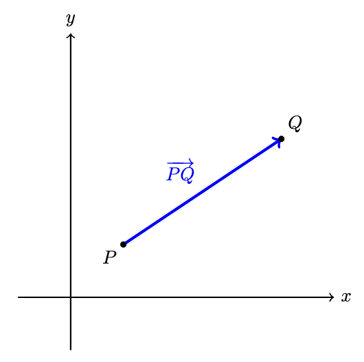
Let’s first define what a vector is in \(\R^2\text{.}\) A vector in \(\R^2\) is an object determined by two points in the plane: an initial point \(P\) (the tail) and a terminal point \(Q\) (the tip). We write
\begin{equation*} \v{v} = \overrightarrow{PQ} \end{equation*}
and we draw \(\v{v}\) as an arrow pointing from \(P\) to \(Q\text{.}\)
Figure 12.1.1. The vector \(\v{v} = \overrightarrow{PQ}\) in \(\R^2\)

Note 12.1.2. Why is \(\v{v}\) bolded but not \(P\) or \(Q\text{?}\)

This is a notation convention. There is a difference between a vector and a point (or scalar). To specify the difference, we usually bold the vector notation.
For example, if you see something like \(\v{u}\text{,}\) then this indicates that \(\v{u}\) is a vector. As a comparison, if you see something like \(u\text{,}\) then this indicates that \(u\) is a scalar (a number).
But why don’t we bold the vector \(\overrightarrow{PQ}\) as \(\v{PQ}\text{,}\) but instead put an arrow on top of it?
That is because the arrow notation specifies the tail and the tip of the vector! There is a difference between \(\overrightarrow{PQ}\) and \(\overrightarrow{QP}\text{!}\) They have the opposite tail and tip, so they point in opposite directions!
Another reason why sometimes we use the arrow notation is because it is super difficult to write in bold font! This is why Richard often writes \(\overrightarrow{\, v\, }\) on the board to indicate the vector \(\v{v}\text{,}\) since he can’t write in bold font easily...
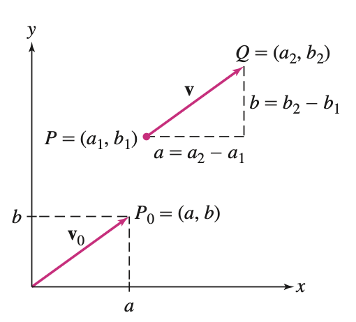
In \(\R^2\text{,}\) each point is represented by an ordered pair of real numbers. Then we can define the components of a vector using the ordered pairs of the two points as follows.

Definition 12.1.3. Components of a Vector.

The components of \(\v{v} = \overrightarrow{PQ}\text{,}\) where \(P = (a_1, b_1)\) and \(Q = (a_2, b_2)\text{,}\) are the quantities
\begin{equation*} a = a_2 - a_1 \quad \text{($x$-component)}\, , \qquad \qquad b = b_2 - b_1 \quad \text{($y$-component)} \end{equation*}
The pair of components is denoted \(\langle a,b \rangle\text{.}\)
P.S.: If you are a linear algebra-ist and want to use the notation of the column vectors instead, be my guest! Just remember that Richard prefers the column vector notation over the sharp-y angle bracket notation (but he is teaching calculus, not linear algebra, so he will have to live with it).

Example 12.1.4.

Find the components of the following vectors with tail \(P\) and tip \(Q\text{.}\) Then sketch the vectors.
  1. \(P_1 = (1,2)\) and \(Q_1 = (4,6)\)
  2. \(P_2 = (-4,-2)\) and \(Q_2 = (-1,2)\)
  3. \(P_3 = (2,-1)\) and \(Q_3 = (-3,-1)\)
  4. \(P_4 = (-2,4)\) and \(Q_4 = (-5,1)\)
Solution.
We can find the components of each vector using the definition:
\begin{equation*} \v{v} = \la a_2 - a_1, b_2 - b_1 \ra \end{equation*}
  1. \(\displaystyle \v{v}_1 = \overrightarrow{P_1Q_1} = \la 4-1, 6-2 \ra = \la 3, 4 \ra\)
  2. \(\displaystyle \v{v}_2 = \overrightarrow{P_2Q_2} = \la -1 - (-4), 2 - (-2) \ra = \la 3, 4 \ra\)
  3. \(\displaystyle \v{v}_3 = \overrightarrow{P_3Q_3} = \la -3 - 2, -1 - (-1) \ra = \la -5, 0 \ra\)
  4. \(\displaystyle \v{v}_4 = \overrightarrow{P_4Q_4} = \la -5 - (-2), 1 - 4 \ra = \la -3, -3 \ra\)
The sketches of the vectors are shown below:
Figure 12.1.5.
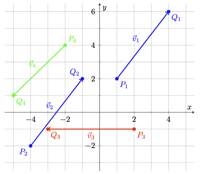
Observe that \(\v{v}_1\) and \(\v{v}_2\) are parallel. Moreover, \(\v{v}_2\) is a translation of \(\v{v}_1\) (i.e., we can obtain \(\v{v}_2\) by sliding \(\v{v}_1\) to the left and down). We call these two vectors equivalent vectors if one is a translation of the other.
In fact, two vectors are equivalent if and only if they have the same components. So instead of studying millions of the same vectors in different locations, we can just study one representative vector for each group of equivalent vectors.
But which location should we choose for the representative vector? To keep things easier, we usually choose the representative vector whose tail is at the origin \((0,0)\text{.}\) Then the tip of the vector is at the coordinate point \((a,b)\text{,}\) where \(\langle a,b \rangle\) are the components of the vector. This is called the position vector.

Example 12.1.6.

Sketch the position vectors of the vectors in the previous example.
Solution.
The vectors in the previous example are
\begin{equation*} \v{v}_1 = \v{v}_2 = \la 3, 4 \ra, \quad \v{v}_3 = \la -5, 0 \ra, \quad \v{v}_4 = \la -3, -3 \ra \end{equation*}
The position vectors are sketched below.
Figure 12.1.7.

Subsection The Attributes of Vectors

When defining a vector, it is important to note its magnitude and the direction.
The magnitude of a vector \(\v{v}\) is the distance from the tail to the tip (aka the length of the vector). This is denoted as \(\|\v{v}\|\text{.}\)
Given a vector \(\v{v} = \langle a,b \rangle\text{,}\) we can determine its magnitude using the Pythagorean Theorem, as demonstrated in the figure below.
Figure 12.1.8. The Magnitude of the vectors \(\v{v}_0\) and \(\v{v}\)
By the Pythagorean Theorem, we have
\begin{align*} \|\v{v}\| \amp= \sqrt{(a_1 - a_2)^2 + (b_1 - b_2)^2} \\ \amp= \sqrt{a^2 + b^2} \end{align*}
The magnitude of a vector is really called the \(\boldsymbol{\ell^2}\) norm or the Euclidean norm of a vector in more advanced math courses. In general, norms must satisfy the following three properties:
  1. \(\|\v{v}\| \geq 0\text{,}\) with \(\|\v{v}\| = 0\) if and only if \(\v{v} = \v{0}\text{.}\)
  2. \(\| \lambda\v{v}\| = |\lambda|\|\v{v}\|\) for all scalars \(\lambda \in \R\text{.}\)
  3. \(\|\v{v} + \v{w}\| \leq \|\v{v}\| + \|\v{w}\|\) for any two vectors \(\v{v}\) and \(\v{w}\text{,}\) with equallity only if \(\v{v} = 0\text{,}\) \(\v{w} = 0\text{,}\) or if \(\v{w} = \lambda\v{v}\) where \(\lambda \geq 0\text{.}\) (This is the famous triangle inequality).
This isn’t a linear algebra or functional analysis class, so we won’t go deeper into norms here. If you are interested, feel free to do more digging on your own (or ask Richard!).

Example 12.1.9.

Find the magnitude of the vectors in the previous examples.
Solution.
The vectors in the previous examples are
\begin{equation*} \v{v}_1 = \v{v}_2 = \la 3, 4 \ra, \quad \v{v}_3 = \la -5, 0 \ra, \quad \v{v}_4 = \la -3, -3 \ra \end{equation*}
Then
\begin{align*} \|\v{v}_1\| \amp= \sqrt{3^2 + 4^2} = \sqrt{25} = 5 \\ \|\v{v}_3\| \amp= \sqrt{(-5)^2 + 0^2} = \sqrt{25} = 5 \\ \|\v{v}_4\| \amp= \sqrt{(-3)^2 + (-3)^2} = \sqrt{18} = 3\sqrt{2} \end{align*}
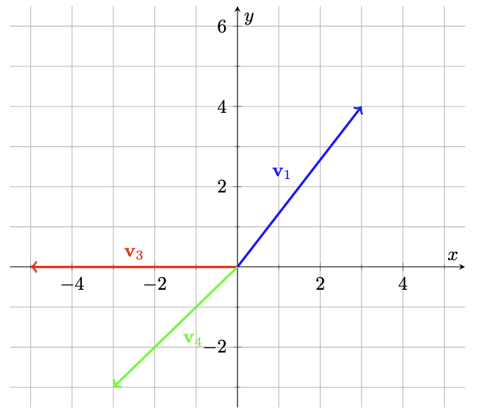
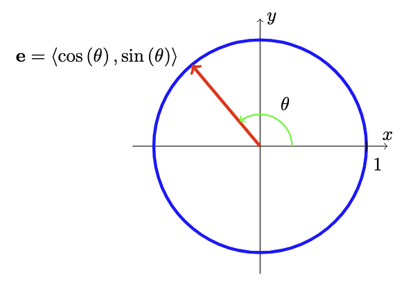
Now let’s discuss the direction of a vector. The direction of a vector tells us where the vector is pointing. We can indicate the direction of a vector by using the vector itself. As you imagine, the magnitude of a vector has nothing to do with its direction, so we sometimes use a unit vector, which is a vector of length \(1\text{,}\) to indicate the direction, when it is not necessary to specify length.
If we have a unit vector whose tail is at the origin, then its tip lies on the unit circle. We usually denote a unit vector by \(\v{e}\text{,}\) defined as
\begin{equation*} \v{e} = \langle \cos(\theta), \sin(\theta)\rangle \end{equation*}
where \(\theta\) is the angle between \(\v{e}\) and the positive \(x\)-axis, indicated in the figure below.
Figure 12.1.10. The unit vector \(\v{e}\) on the unit circle
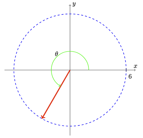
But what if we are given an arbitrary non-zero vector and we want to find a unit vector in the same direction? One way to do so is to divide the vector by its magnitude (multiplying a positive scalar doesn’t change the direction of a vector). That is, given \(\v{v}\text{,}\) the unit vector in the direction of \(\v{v}\) is
\begin{equation*} \v{e_v} = \frac{1}{\|\v{v}\|}\v{v} \end{equation*}

A quick proof to show that \(\v{e_v}\) is a unit vector.

Let \(\v{v}\) be a non-zero vector. Then \(\|\v{v}\| \gt 0\text{.}\) This implies that
\begin{align*} \|\v{e_v}\| \amp= \left\|\frac{1}{\|\v{v}\|}\v{v}\right\| \\ \amp= \left|\frac{1}{\|\v{v}\|}\right| \|\v{v}\| \amp\amp\text{by the second norm property} \\ \amp= \frac{1}{\|\v{v}\|}\|\v{v}\| \amp\amp\text{since } \frac{1}{\|\v{v}\|} \gt 0 \\ \amp= 1 \end{align*}
Hence, \(\v{e_v}\) is a unit vector.
When we are given the magnitude of a vector and its direction as the angle \(\theta\text{,}\) we can find the components of the vector as follows:
\begin{equation*} \v{v} = \la v_1, v_2 \ra = \|\v{v}\|\v{e_v} = \|\v{v}\|\la \cos(\theta), \sin(\theta) \ra = \la \|\v{v}\|\cos(\theta), \|\v{v}\|\sin(\theta) \ra \end{equation*}

Example 12.1.11.

Find the vector with magnitude \(6\) and make an angle of \(\dfrac{4\pi}{3}\) with the positive \(x\)-axis.
Hint. If you want to see what the vector looks like...
The goal of the question is to find the length of the red vector in the figure below.
Figure 12.1.12.
Solution.
We can first find the unit vector in the direction of the vector:
\begin{equation*} \v{e_v} = \la \cos\lp \frac{4\pi}{3} \rp, \sin\lp \frac{4\pi}{3} \rp \ra = \la -\frac{1}{2}, -\frac{\sqrt{3}}{2} \ra \end{equation*}
Then the vector with magnitude \(6\) in the same direction is
\begin{equation*} \v{v} = \la 6 \cdot \left(-\frac{1}{2}\right), 6 \cdot \left(-\frac{\sqrt{3}}{2}\right) \ra = \la -3, -3\sqrt{3} \ra \end{equation*}
Observe that we essentially multiplied the unit vector (a vector) by the magnitude (a scalar) to obtain the desired vector. This is one of the two operations in vector algebra, which we will discuss in the next section.

Subsection Vector Algebra

Vectors live in a place called the vector space. Usually, two operations are defined in a vector space, and they are vector addition and scalar multiplication. We will discuss these two operations in this section.
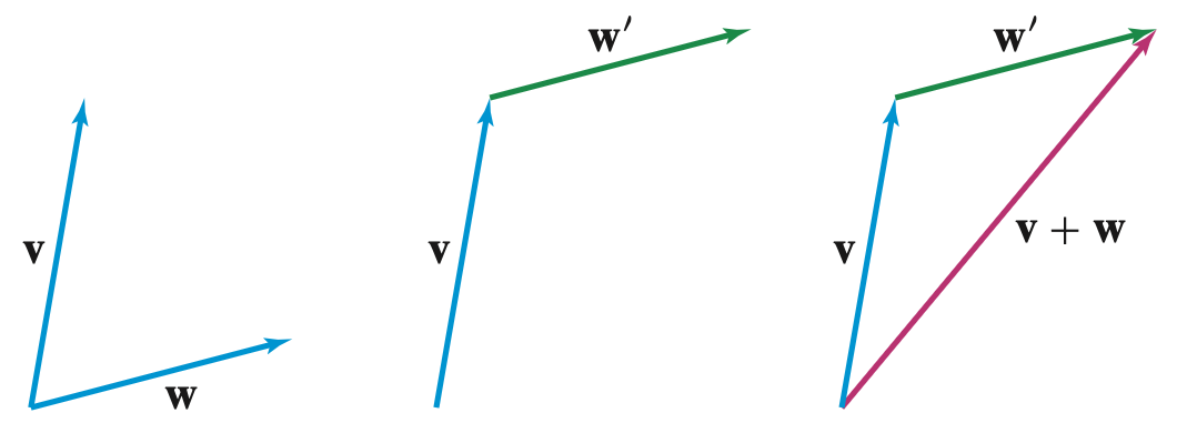
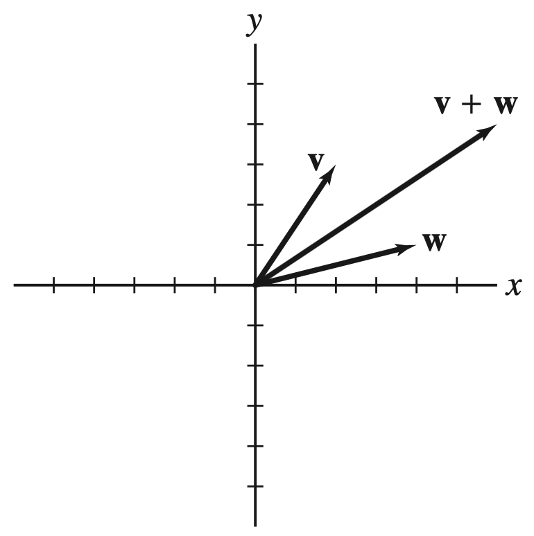
Vector addition tells us how to add two vectors together. Geometrically speaking, we can imagine a vector as the movement from the tail to the tip. Then adding two vectors means performing the movements one after another. That is, we will need to find the equivalent vector of the second vector whose tail is at the tip of the first vector, and the resulting vector is the vector from the tail of the first vector to the tip of the second vector. This is sometimes referred to as the Triangle Law.
Figure 12.1.13. Vector Addition using the Triangle Law
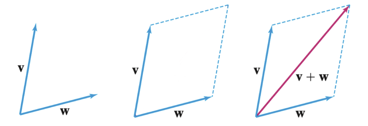
But sometimes we are given the position vectors and their tails are both at the origin (or at the same point). Alternatively, rather than finding the equivalent vector of the second vector, we can construct a parallelogram using the two vectors as adjacent sides, and the resulting vector is the diagonal of the parallelogram starting from the common tail of the two vectors. This is called the Parallelogram Law.
Figure 12.1.14. Vector Addition using the Parallelogram Law
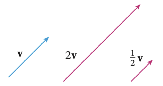
Now let’s look at scalar multiplication. The term scalar refers to a real number. That is, scalar multiplication tells us how to multiply a vector by a real number. The scalar will "scale" or "resize" the vector.
When the scalar is positive, the resulting vector points in the same direction, and the size of the vector is scaled by the scalar.
Figure 12.1.15. Vector Addition using the Parallelogram Law
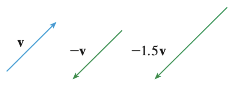
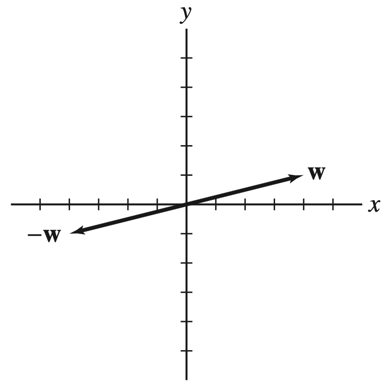
When the scalar is negative, the resulting vector points in the opposite direction, and the size of the vector is scaled by the absolute value of the scalar.
Figure 12.1.16. Vector Multiplication by a Negative Scalar
But what if the scalar is zero? We can quickly see that the magnitude of the resulting vector is zero, so the resulting vector is the zero vector, denoted by \(\v{0}\text{.}\) We can imagine the zero vector has the tail and tip at the same point, which means it doesn’t have a specific direction. Alternatively, we can say that the zero vector points in all directions.
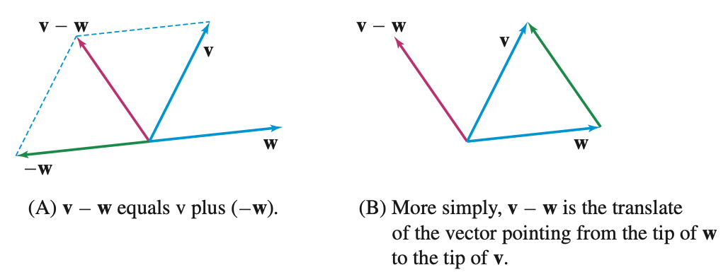
Once we have vector addition and scalar multiplication defined, we can subtract two vectors. Recall subtraction is really the same thing as adding the opposite. That is,
\begin{equation*} \v{v} - \v{w} = \v{v} + (-\v{w}) \end{equation*}
Graphically, we can find \(\v{v} - \v{w}\) as follows:
Figure 12.1.17. Vector Subtraction
But we work with components of vectors as well... How do we perform these operations using components? It turns out that vector addition and scalar multiplication can be performed component-wise.

Example 12.1.19.

Calculate \(\la -\dfrac{1}{2},\dfrac{5}{3} \ra + \la 3,\dfrac{10}{3} \ra\text{.}\)
Solution.
The vector sum is
\begin{equation*} \la -\dfrac{1}{2},\dfrac{5}{3} \ra + \la 3,\dfrac{10}{3} \ra = \la -\dfrac{1}{2} + 3, \dfrac{5}{3} + \dfrac{10}{3} \ra = \la \dfrac{5}{2}, 5 \ra \end{equation*}
Observe that vector operations are (kind of) similar to operations with numbers component-wise. Then some properties of number operations also hold for vector operations.

Subsubsection Linear Combinations of Vectors

Given two vectors \(\v{v}\) and \(\v{w}\text{,}\) we define a linear combination of them as a vector of the form
\begin{equation*} r\v{v} + s\v{w} \end{equation*}
where \(r\) and \(s\) are scalars. Linear combinations are the fundamental mechanism for "building" new vectors from existing ones.
Example 12.1.21.
Express \(\v{u}\) as a linear combination \(\v{u} = r\v{v} + s\v{w}\text{,}\) where
\begin{equation*} \v{u} = \la 6,-2 \ra , \qquad \v{v} = \la 1,1 \ra \quad \text{and} \quad \v{w} = \la 1,-1 \ra \end{equation*}
Then sketch \(\v{u}\text{,}\) \(\v{v}\text{,}\) \(\v{w}\text{,}\) and the parallelogram formed by \(r\v{v}\) and \(s\v{w}\text{.}\)
Hint.
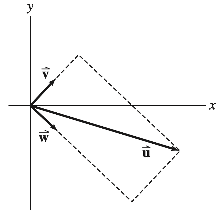
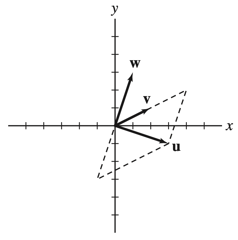
Consider the vectors \(\v{v}\) and \(\v{w}\) are the two building blocks that we can use to construct the vector \(\v{u}\text{.}\) The moves we can do are the scalar multiplications (to resize the building blocks) and the vector addition (to combine the building blocks).
So, the question here is: how should we resize the building blocks \(\v{v}\) and \(\v{w}\) such that when we combine them together, we get the desired vector \(\v{u}\text{?}\)
Solution.
Using the definition of linear combinations, there are two scalars \(r\) and \(s\) such that
\begin{align*} \v{u} = \la 6,-2 \ra = r\v{v} + s\v{w} \amp= r\la 1,1 \ra + s\la 1,-1 \ra \\ \amp= \la r,r \ra + \la s,-s \ra \\ \amp= \la r + s, r - s \ra \end{align*}
This implies that
\begin{equation*} \begin{cases} r + s = 6 \\ r - s = -2 \end{cases} \end{equation*}
Solving this system of equations, we obtain \(r = 2\) and \(s = 4\text{.}\) Hence, the linear combination is
\begin{equation*} \v{u} = 2\v{v} + 4\v{w} \end{equation*}
The sketches of the vectors and the parallelogram are shown below.
Figure 12.1.22.
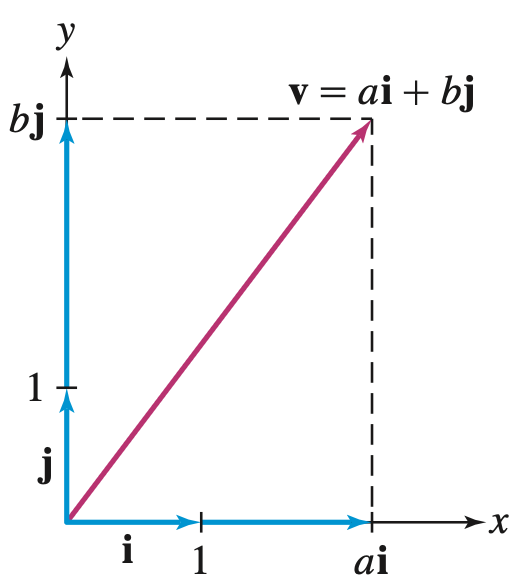
One of the reasons why linear combinations are important is that we can decompose vectors into linear combinations of other vectors. Usually, we want to decompose vectors into linear combinations of the simplest vectors possible. In \(\R^2\text{,}\) the simplest vectors are the standard basis vectors, defined as
\begin{equation*} \v{i} = \la 1,0 \ra \quad \text{and} \quad \v{j} = \la 0,1 \ra \end{equation*}
Any vector in \(\R^2\) can be expressed as a linear combination of these two vectors. Or using fancy linear algebra terminology, the set \(\{\v{i},\v{j}\}\) spans the vector space \(\R^2\text{.}\)
Figure 12.1.23. Linear Combination using the standard basis vectors in \(\R^2\)
Example 12.1.24.
Calculate the linear combination \(-\dfrac{3}{2}\v{i} + 5\lp \dfrac{1}{2}\v{j} - \dfrac{1}{2}\v{i} \rp\)
Hint.
The building blocks here are the standard basis vectors \(\v{i} = \la 1,0 \ra\) and \(\v{j} = \la 0,1 \ra\text{.}\) So we will need to perform scalar multiplications and vector additions to obtain the resulting vector.
Solution.
\begin{align*} -\dfrac{3}{2}\v{i} + 5\lp \dfrac{1}{2}\v{j} - \dfrac{1}{2}\v{i} \rp \amp= -\dfrac{3}{2}\v{i} + \dfrac{5}{2}\v{j} - \dfrac{5}{2}\v{i} \\ \amp= -\dfrac{8}{2}\v{i} + \dfrac{5}{2}\v{j} \\ \amp= -4\la 1,0 \ra + \dfrac{5}{2}\la 0,1 \ra \\ \amp= \la -4,0 \ra + \la 0, \dfrac{5}{2} \ra \\ \amp= \la -4, \dfrac{5}{2} \ra \end{align*}

Subsection Applications of Vectors

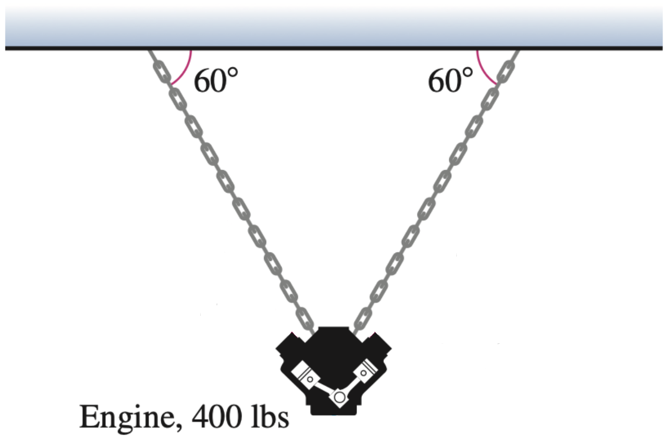
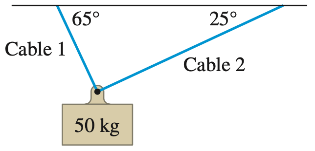
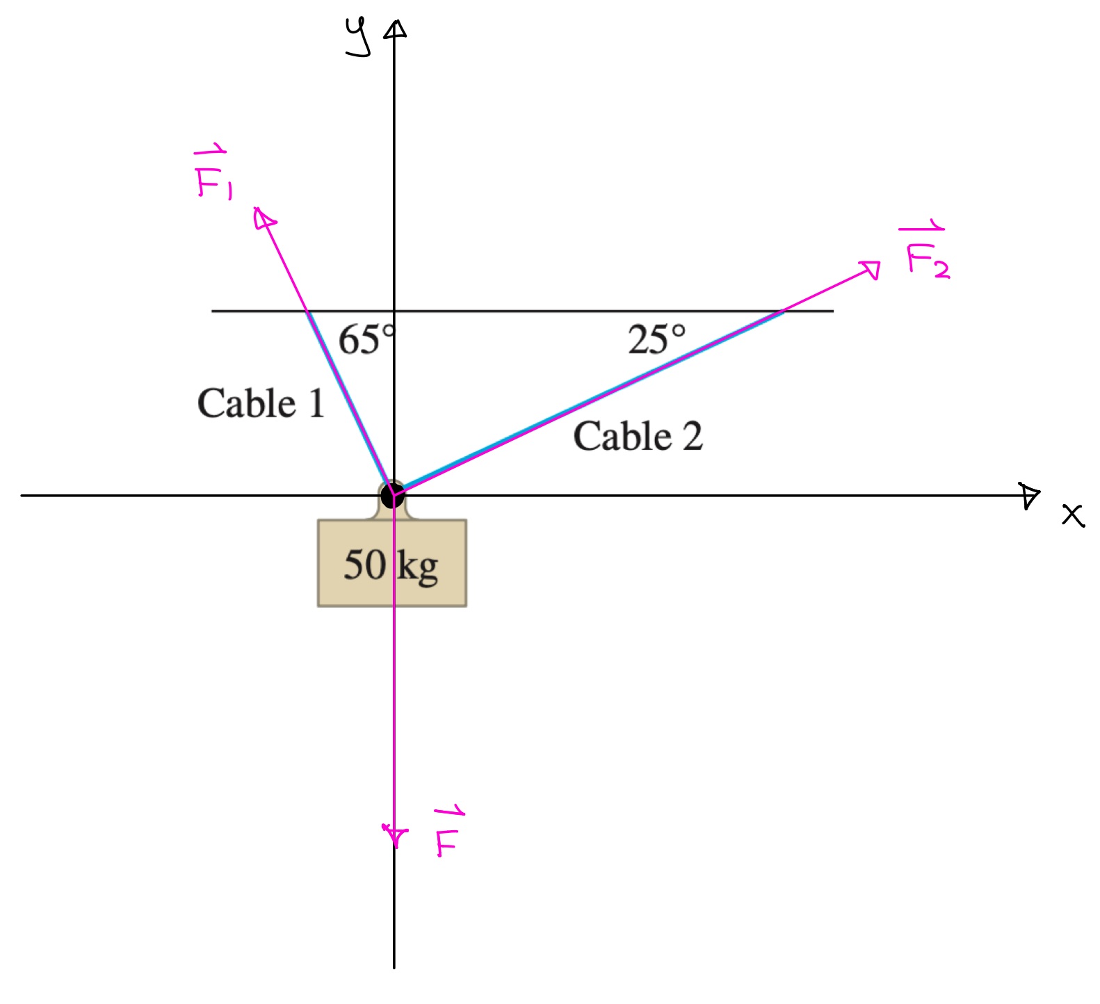
Vectors are widely used in various fields, including physics, engineering, computer science, and more. They are particularly useful in representing quantities that have both magnitude and direction, such as velocity, force, and acceleration. In this section, we will explore a basic application of vectors: force vectors.

Example 12.1.25. Force Vectors.

A 400-lb engine is suspended from two chains that form 60Β° angles with a horizontal ceiling. How much weight does each chain support?
Figure 12.1.26.
Hint.
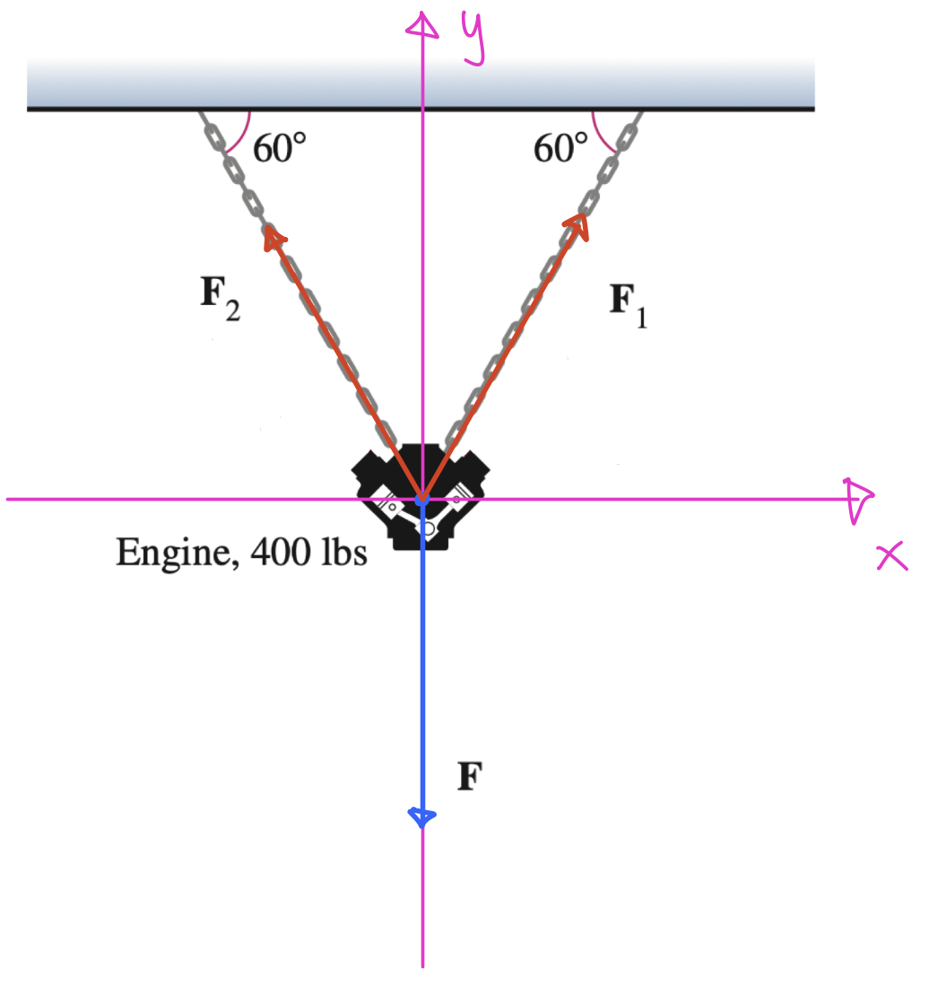
Let \(\v{F}_1\) and \(\v{F}_2\) denote the forces exerted by the chains on the engine and let \(\v{F}_3\) be the downward force due to the weight of the engine. Then we can place the origin at the point where the engine is located and construct a Cartesian coordinate plane.
Then we can draw the vectors \(\v{F}_1\text{,}\) \(\v{F}_2\text{,}\) and \(\v{F}_3\text{.}\) Can we find the components of these vectors?
Since the engine is stationary, the forces must be balanced. That is, adding these three vectors together must give us the zero vector.
Solution.
Following the setup in the hint, we can construct a Cartesian coordinate plane with the origin at the engine. Then the vectors are
\begin{equation*} \v{F}_1 = \la \|\v{F}_1\| \cos\lp 60^\circ \rp, \|\v{F}_1\| \sin\lp 60^\circ \rp \ra = \la \frac{1}{2}\|\v{F}_1\|, \frac{\sqrt{3}}{2}\|\v{F}_1\| \ra \end{equation*}
\begin{equation*} \v{F}_2 = \la \|\v{F}_2\| \cos\lp 120^\circ \rp, \|\v{F}_2\| \sin\lp 120^\circ \rp \ra = \la -\frac{1}{2}\|\v{F}_2\|, \frac{\sqrt{3}}{2}\|\v{F}_2\| \ra \end{equation*}
\begin{equation*} \v{F}_3 = \la 0, -400 \ra \end{equation*}
Figure 12.1.27.
Since the engine is stationary, we have
\begin{equation*} \v{F}_1 + \v{F}_2 + \v{F}_3 = \v{0} \end{equation*}
This implies that
\begin{equation*} \la \frac{1}{2}\|\v{F}_1\| - \frac{1}{2}\|\v{F}_2\|, \frac{\sqrt{3}}{2}\|\v{F}_1\| + \frac{\sqrt{3}}{2}\|\v{F}_2\| - 400 \ra = \la 0,0 \ra \end{equation*}
Equating the components, we obtain the system of equations:
\begin{equation*} \begin{cases} \dfrac{1}{2}\|\v{F}_1\| - \dfrac{1}{2}\|\v{F}_2\| = 0 \\ \dfrac{\sqrt{3}}{2}\|\v{F}_1\| + \dfrac{\sqrt{3}}{2}\|\v{F}_2\| - 400 = 0 \end{cases} \end{equation*}
Solving this system, we find that \(\|\v{F}_1\| = \|\v{F}_2\| = \dfrac{400}{\sqrt{3}} \approx 230.94\) lbs.
Hence, each chain must be able to support a weight of approximately 230.94 lbs.

Worksheet Assigned Problems for Section 12.1

The problems listed below are assigned to be included in your problem set portfolio. Note that a specific selection of these problems will also form the written homework assignments. I recommend working through all of them to ensure a solid grasp of the material. Reach out to Richard for help if you get stuck or have any questions.
The solutions will be posted after the written homework due dates. If you have any questions about your work, talk to Richard and he is happy to discuss the process with you.

12.1.5.

Find the components of the unit vector \(\v{u}\) in the figure below.
Figure 12.1.28.
Solution.
Since \(\v{u}\) makes an angle of \(45^\circ\) with the positive \(x\)-axis, its components are
\begin{equation*} \|\v{u}\| \la \cos\lp 45^\circ\rp, \sin\lp 45^\circ\rp \ra = \|\v{u}\| \la \frac{\sqrt{2}}{2}, \frac{\sqrt{2}}{2}\ra \end{equation*}

12.1.11.

Find the components of \(\overrightarrow{PQ}\text{,}\) where \(P=(1,-7)\) and \(Q=(0,17)\text{.}\)
Solution.
Using the definition of components of a vector, we have
\begin{equation*} \overrightarrow{PQ} = \la 0 - 1, 17 - (-7) \ra = \la -1, 24 \ra \end{equation*}

12.1.19.

Calculate \(\la 2e, 1 - 2\pi\ra - \la 2e - \pi, 8 - 2\pi\ra\text{.}\)
Solution.
Using vector algebra, we obtain
\begin{align*} \la 2e, 1 - 2\pi\ra - \la 2e - \pi, 8 - 2\pi\ra \amp= \la 2e - (2e - \pi), (1 - 2\pi) - (8 - 2\pi) \ra \\ \amp= \la \pi, -7 \ra \end{align*}

12.1.23.

Sketch \(2\v{v}\text{,}\) \(-\v{w}\text{,}\) \(\v{v} + \v{w}\text{,}\) and \(2\v{v} - \v{w}\) in the following figure.
Figure 12.1.29.
Solution.
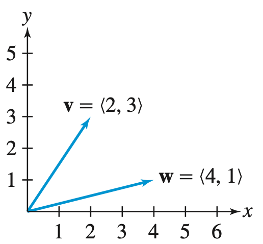
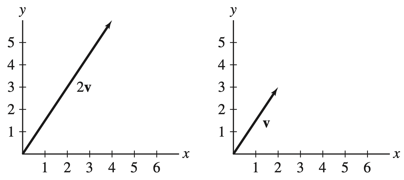
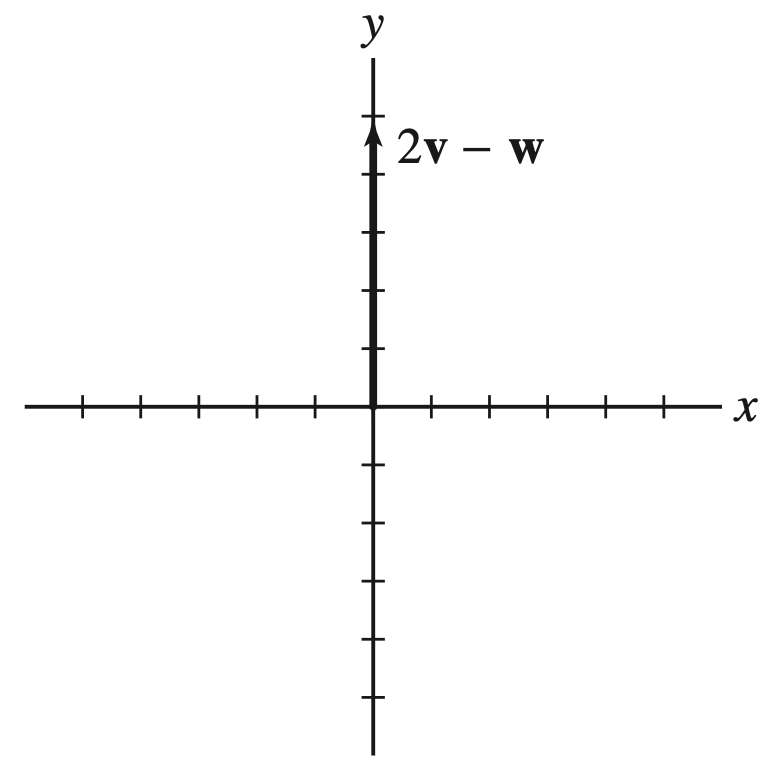
The scalar multiple \(2\v{v}\) points in the same direction as \(\v{v}\) and its length is twice the length of \(\v{v}\text{.}\) It is the vector \(2\v{v} = \la 4, 6 \ra\text{.}\)
Figure 12.1.30. The sketch of \(\v{v}\) and \(2\v{v}\text{.}\)
\(-\v{w}\) has the same length as \(\v{w}\) but points to the opposite direction. It is the vector \(-\v{w} = \la -4, -1 \ra\text{.}\)
Figure 12.1.31. The sketch of \(\v{w}\) and \(-\v{w}\text{.}\)
The vector sum \(\v{v} + \v{w}\) is the vector:
\begin{equation*} \v{v} + \v{w} = \la 2, 3 \ra + \la 4, 1 \ra = \la 6, 4 \ra \end{equation*}
The vector is shown in the following figure:
Figure 12.1.32. The sketch of \(\v{v}\text{,}\) \(\v{w}\text{,}\) and \(\v{v} + \v{w}\text{.}\)
The vector \(2\v{v} - \v{w}\) is the vector:
\begin{equation*} 2\v{v} - \v{w} = 2\la 2, 3 \ra - \la 4, 1 \ra = \la 4, 6 \ra - \la 4, 1 \ra = \la 0, 5 \ra \end{equation*}
It is shown next:
Figure 12.1.33. The sketch of \(\v{v}\text{,}\) \(\v{w}\text{,}\) and \(2\v{v} - \v{w}\text{.}\)

12.1.25.

Sketch \(\v{v} = \langle 0,2\rangle\text{,}\) \(\v{w} = \langle -2, 4\rangle\text{,}\) \(3\v{v} + \v{w}\text{,}\) and \(2\v{v} - 2\v{w}\text{.}\)
Solution.
We compute the vectors and then sketch them:
\begin{equation*} 3\v{v} + \v{w} = 3\la 0, 2 \ra + \la -2, 4 \ra = \la 0, 6 \ra + \la -2, 4 \ra = \la -2, 10 \ra \end{equation*}
\begin{equation*} 2\v{v} - 2\v{w} = 2\la 0, 2 \ra - 2\la -2, 4 \ra = \la 0, 4 \ra - \la -4, 8 \ra = \la 4, -4 \ra \end{equation*}
Figure 12.1.34. The sketch of \(\v{v}, \v{w}, 3\v{v} + \v{w},\) and \(2\v{v} - 2\v{w}\text{.}\)

12.1.35.

Are \(\overrightarrow{AB}\) and \(\overrightarrow{PQ}\) parallel if \(A=(1,1)\text{,}\) \(B=(3,4)\text{,}\) \(P=(1,1)\text{,}\) and \(Q=(7,10)\text{?}\) And if so, do they point in the same direction?
Solution.
We compute the vectors \(\overrightarrow{AB}\) and \(\overrightarrow{PQ}\text{:}\)
\begin{equation*} \overrightarrow{AB} = \la 3 - 1, 4 - 1 \ra = \la 2, 3 \ra \end{equation*}
\begin{equation*} \overrightarrow{PQ} = \la 7 - 1, 10 - 1 \ra = \la 6, 9 \ra \end{equation*}
Since \(\overrightarrow{AB} = \dfrac{1}{3} \la 6, 9 \ra\text{,}\) the vectors are parallel and point in the same direction.

Exercise Group.

In the following exercises, find the given vector.
12.1.43.
Unit vector \(\v{e_v}\text{,}\) where \(\v{v} = \langle 3, 4 \rangle\text{.}\)
Solution.
We find the length of \(\v{v} = \la 3, 4 \ra\text{:}\)
\begin{equation*} \|\v{v}\| = \sqrt{3^2 + 4^2} = 5 \end{equation*}
Then the unit vector in the direction of \(\v{v}\) is
\begin{equation*} \v{e_v} = \frac{1}{5} \la 3, 4 \ra = \la \frac{3}{5}, \frac{4}{5} \ra \end{equation*}
12.1.45.
Vector of length \(4\) in the direction of \(\v{u} = \langle -1, -1 \rangle\text{.}\)
Solution.
We first find the unit vector in the direction of \(\v{u}\text{:}\)
\begin{equation*} \v{e_u} = \frac{1}{\|\v{u}\|} \v{u} = \frac{1}{\sqrt{(-1)^2 + (-1)^2}} \la -1, -1 \ra = \la -\frac{1}{\sqrt{2}}, -\frac{1}{\sqrt{2}} \ra \end{equation*}
We now multiply \(\v{e_u}\) by \(4\) to obtain the desired vector:
\begin{equation*} 4\v{e_u} = 4 \la -\frac{1}{\sqrt{2}}, -\frac{1}{\sqrt{2}} \ra = \la -\frac{4}{\sqrt{2}}, -\frac{4}{\sqrt{2}} \ra = \la -2\sqrt{2}, -2\sqrt{2} \ra \end{equation*}
12.1.49.
Unit vector \(\v{e}\) making an angle of \(\dfrac{4\pi}{7}\) with the \(x\)-axis.
Solution.
The unit vector \(\v{e}\) is the following vector:
\begin{equation*} \v{e} = \la \cos\lp \frac{4\pi}{7}\rp, \sin\lp \frac{4\pi}{7}\rp \ra = \la -0.22, 0.97\ra \end{equation*}

12.1.61.

Calculate the linear combination \(\lp 3\v{i} + \v{j} \rp - 6\v{j} + 2\lp \v{j} - 4\v{i} \rp\)
Solution.
\begin{align*} \lp 3\v{i} + \v{j} \rp - 6\v{j} + 2\lp \v{j} - 4\v{i} \rp \amp= \lp 3\la 1, 0\ra + \la 0, 1\ra \rp - 6\la 0, 1\ra + 2\lp \la 0, 1\ra - 4\la 1, 0\ra \rp \\ \amp= \lp \la 3, 0\ra + \la 0, 1\ra \rp - \la 0, 6\ra + 2\lp \la 0, 1\ra - \la 4, 0\ra \rp \\ \amp= \la 3, 0\ra + \la 0, 1\ra - \la 0, 6\ra + \la 0, 2\ra - \la 8, 0\ra \\ \amp= \la 3 + 0 - 0 + 0 - 8, 0 + 1 - 6 + 2 - 0 \ra \\ \amp= \la -5, -3 \ra \end{align*}

12.1.65.

Express \(\v{u}\) as a linear combination \(\v{u} = r\v{v} + s\v{w}\text{,}\) where
\begin{equation*} \v{u} = \langle 3, -1 \rangle; \qquad\qquad \v{v} = \langle 2, 1 \rangle \quad \text{and} \quad \v{w} = \langle 1, 3 \rangle. \end{equation*}
Then sketch \(\mathbf{u}, \mathbf{v},\mathbf{w}\text{,}\) and the parallelogram formed by \(r\v{v}\) and \(s\v{w}\text{.}\)
Solution.
We have
\begin{equation*} \v{u} = \la 3, -1 \ra = r\v{v} + s\v{w} = r\la 2, 1 \ra + s\la 1, 3 \ra \end{equation*}
which becomes the system of equations
\begin{equation*} \begin{cases} 3 = 2r + s \\ -1 = r + 3s \end{cases} \end{equation*}
Solving the above system of equations, we obtain \(r = 2\) and \(s = -1\text{.}\)
Hence, the linear combination is
\begin{equation*} \v{u} = \la 3, -1 \ra = 2\la 2, 1\ra - 1\la 1, 3 \ra \end{equation*}
The sketch is shown below.
Figure 12.1.35. The sketch of \(\v{u}, \v{v}, \v{w}\) and the parallelogram formed by \(r\v{v}\) and \(s\v{w}\text{.}\)

12.1.67.

Calculate the magnitude of the force on cables 1 and 2 shown in the figure below.
Figure 12.1.36.
Solution.
The three forces acting on the point \(P\) are:
  • The force \(\v{F}\) of magnitude \(50\) lb that acts vertically downward.
  • The forces \(\v{F}_1\) and \(\v{F}_2\) that act through cables 1 and 2 respectively.
The diagram below shows the vectors representing these forces.
Figure 12.1.37.
Since the point \(P\) is not in motion, we have
\begin{equation*} \v{F}_1 + \v{F}_2 + \v{F} = \v{0} \end{equation*}
We compute the forces. Let \(\|\v{F}_1\| = f_1\) and \(\|\v{F}_2\| = f_2\text{.}\) We have
\begin{align*} \v{F}_1 \amp= f_1 \la \cos(115^\circ), \sin(115^\circ) \ra = f_1 \la -0.423, 0.906 \ra \\ \v{F}_2 \amp= f_2 \la \cos(25^\circ), \sin(25^\circ) \ra = f_2 \la 0.906, 0.423 \ra \\ \v{F} \amp= \la 0, -50 \ra \end{align*}
Substituting the forces into the equation gives
\begin{align*} f_1 \la -0.423, 0.906 \ra + f_2 \la 0.906, 0.423 \ra + \la 0, -50 \ra \amp= \v{0}\\ \la -0.423 f_1 + 0.906 f_2, 0.906 f_1 + 0.423 f_2 - 50 \ra \amp= \la 0, 0 \ra \end{align*}
We equate corresponding components and get
\begin{equation*} \begin{cases} -0.423 f_1 + 0.906 f_2 = 0 \\ 0.906 f_1 + 0.423 f_2 - 50 = 0 \end{cases} \end{equation*}
Solving the above system of equations, we obtain \(f_1 = 45.29\) and \(f_2 = 21.16\text{.}\)
We conclude that the magnitude of the force on cable 1 is \(f_1 = 45.29\) lb and the magnitude of the force on cable 2 is \(f_2 = 21.16\) lb.