Objectives
After this section, students will be able to:
-
evaluate functions of two or more variables and use correct functional notation.
-
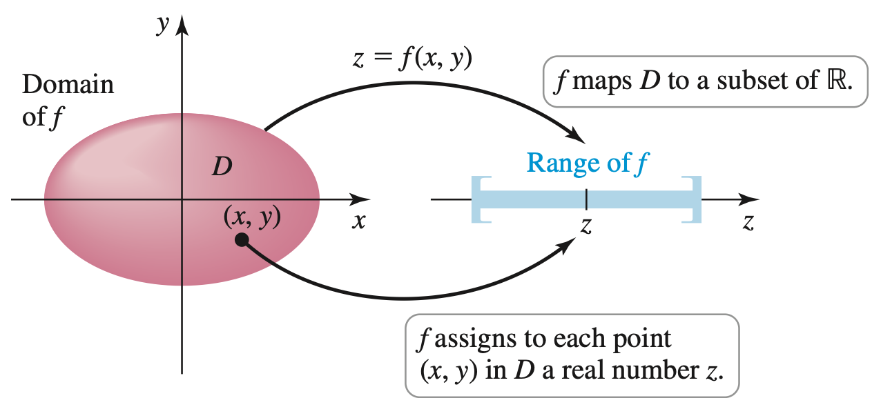
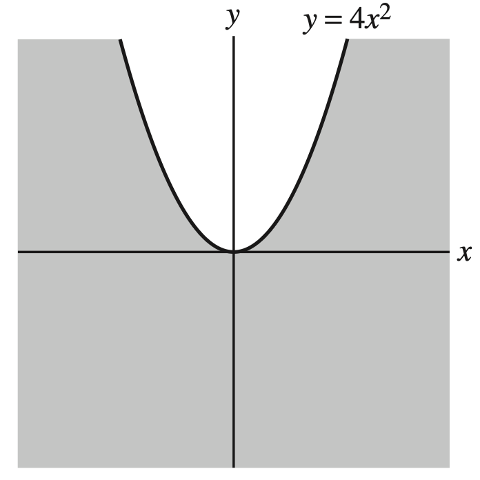
determine and sketch the domain of a function of two variables.
-
determine the range of basic functions of two variables.
-
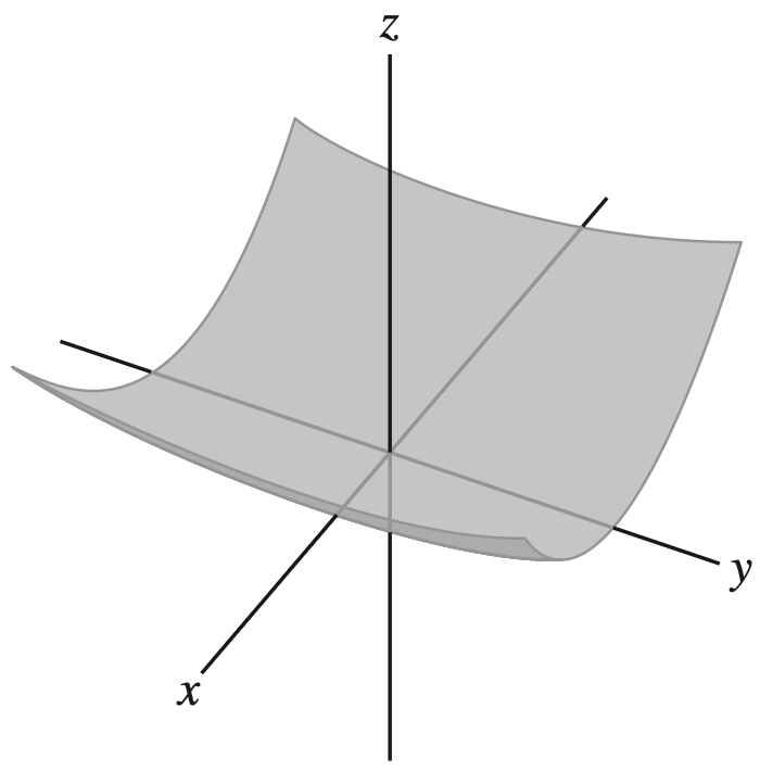
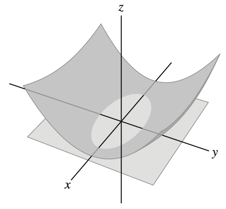
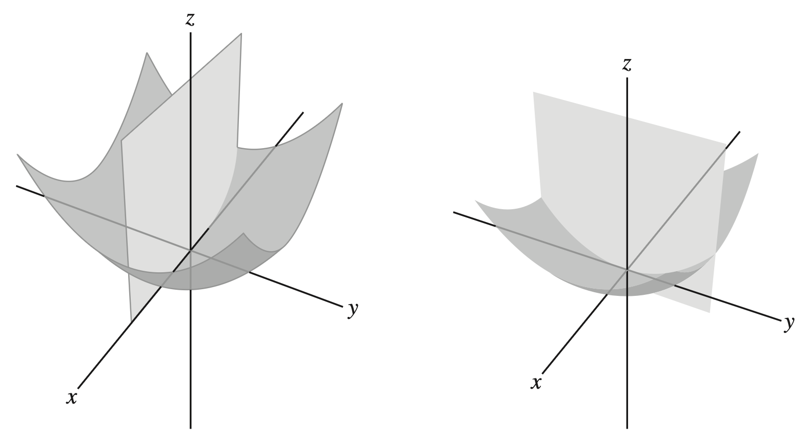
analyze the shape of a surface using traces.
-
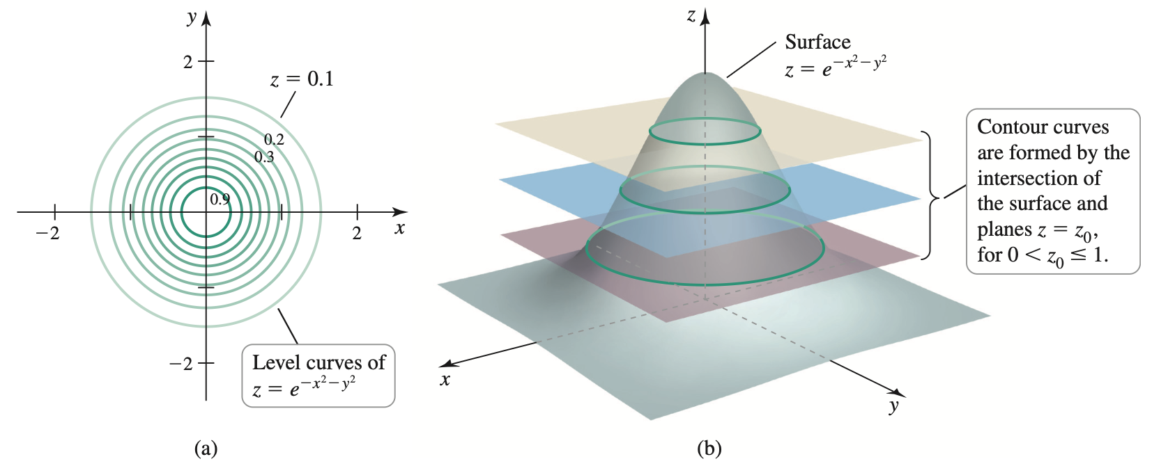
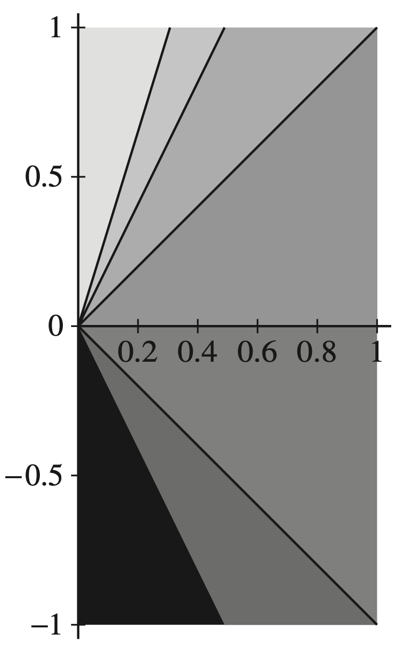
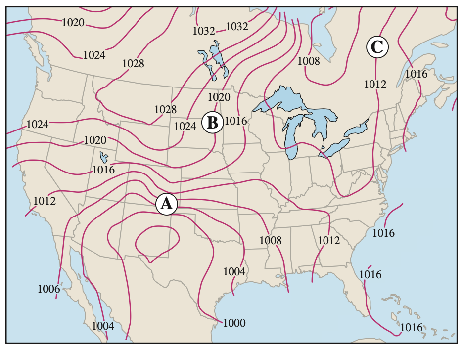
sketch and interpret level curves and contour maps to visualize functions of two variables.
-
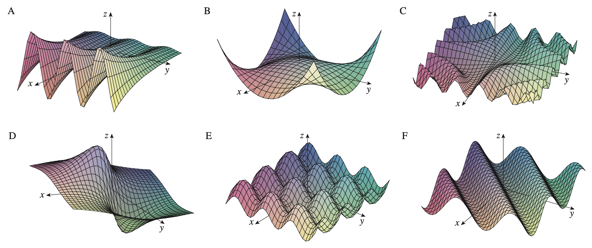
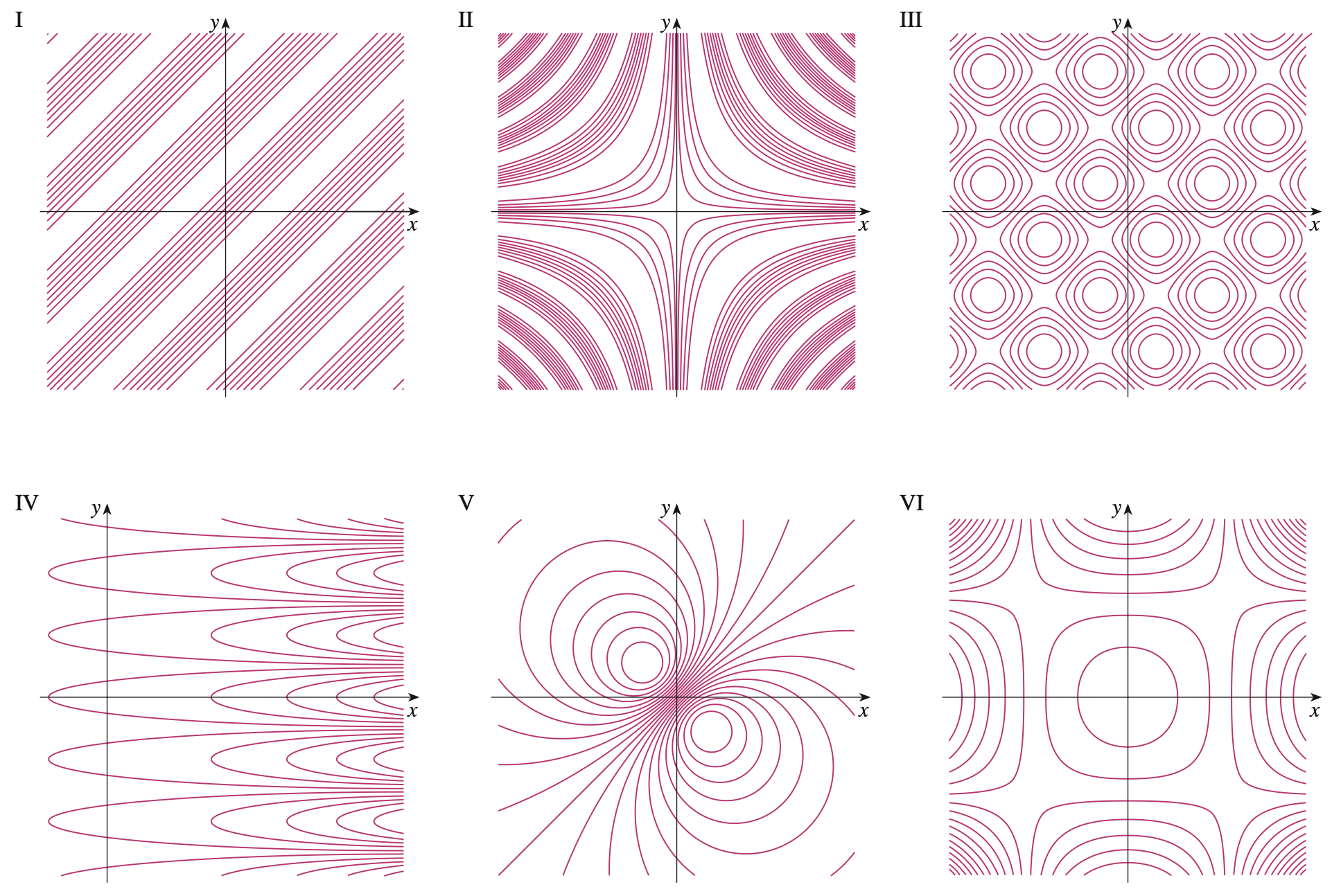
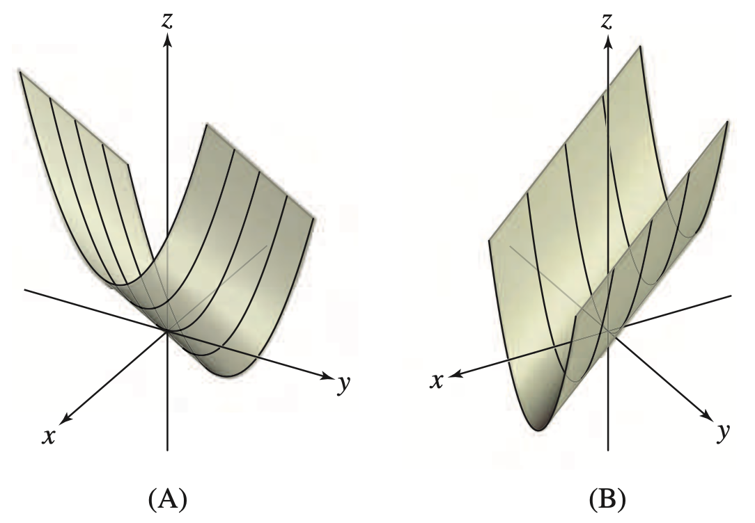
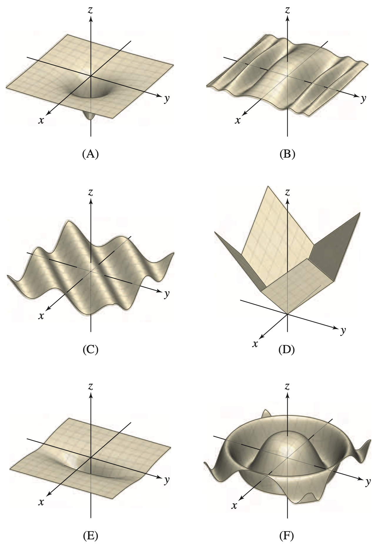
match algebraic equations of functions to their corresponding 3D graphs and contour maps.
-
extend the concept of level curves to describe functions of three variables using level surfaces.