
Section 13.4 Curvature

In this section, we introduce the concept of curvature. Intuitively, curvature measures how sharply a curve bends at a given point.
Long story short, curvature measures how "curvy" a curve is at a given point (aka how much a curve bends). With this idea, we can quickly determine that a line has zero curvature everywhere.
There are several formulas for curvature, each useful in different contexts.

Subsection Mathematical Definition of Curvature

Let’s think about how to define curvature mathematically. Intuitively, curvature measures how quickly the direction of the tangent vector changes as we move along the curve. The faster the tangent vector changes direction, the higher the curvature.
Figure 13.4.1. Curvature is large where the unit tangent vector changes direction quickly.
Well there comes two problems to address here: (1) why using the unit tangent vector, but not just some tangent vector, and (2) how do we measure "how quickly" the unit tangent vector changes direction?
The first question is easier to answer. If we used a non-unit tangent vector, then the magnitude of the tangent vector would affect our measurement of curvature. Since we only care about the direction of the tangent vector when measuring curvature, we use the unit tangent vector. The unit tangent vector, denoted \(\v{T}(t)\text{,}\) is defined as
\begin{equation*} \v{T}(t) = \frac{\v{r}'(t)}{\| \v{r}'(t)\|} \end{equation*}
This formula is just the normalized version of the tangent vector \(\v{r}'(t)\text{.}\)
Now the second question is a bit more subtle. By saying "how quickly" the unit tangent vector changes direction, this suggests we should look at the derivative of the unit tangent vector with respect the arc length, \(s\text{.}\) Hence, the derivative we want is \(\dfrac{d\v{T}}{ds}\text{.}\)
Figure 13.4.2.
However, this derivative isn’t very perfect to measure curvature yet. Recall that the derivative \(\dfrac{d\v{T}}{ds}\) is a vector, but we just want a scalar value to represent curvature. The easiest fix is just to take the magnitude of this vector and call it our curvature!

Definition 13.4.3. Curvature.

Let \(\v{r}(s)\) be an arc length parametrization and \(\v{T}\) the unit tangent vector. The curvature of the underlying curve at \(\v{r}(s)\) is the quantity (denoted by a lowercase Greek letter "kappa")
\begin{equation*} \kappa(s) = \left\| \frac{d\v{T}}{ds} \right\| \end{equation*}
To sum up, curvature is the magnitude of the rate of change of the unit tangent vector \(\v{T}\) with respect to distance traveled \(s\) along the curve.

Note 13.4.4. But Richard... Why using an arc length parametrization?

The short answer is because it makes the definition of curvature cleaner.
What makes an arc length parametrization special is that every velocity vector \(\v{r}'(s)\) has the length of \(1\text{.}\) So we don’t have to worry about the speed of the parametrization affecting our measurement of curvature.

Example 13.4.5.

Compute the curvature of a circle of radius \(R\text{.}\)
Hint.
Feel free to assume that the circle is centered at the origin to make the parametrization easier, since the location of the circle should not affect its curvature.
Then a paramatrization of the circle is
\begin{equation*} \v{r}(t) = \la R\cos(t), R\sin(t) \ra \end{equation*}
Solution.
To find the curvature using the formula, we first need to find an arc length parametrization of the circle.
The arc length function is given by
\begin{align*} s = g(t) = \int_0^t \| \v{r}'(u) \| du \amp= \int_0^t \| \la -R\sin(u), R\cos(u) \ra \| du \\ \amp= \int_0^t R du = Rt \end{align*}
This implies that
\begin{equation*} t = g^{-1}(s) = \frac{s}{R} \end{equation*}
Therefore, the arc length parametrization is
\begin{equation*} \v{r}_1(s) = \v{r}\lp g^{-1}(s)\rp = \v{r}\left(\frac{s}{R}\right) = \la R\cos\left(\frac{s}{R}\right), R\sin\left(\frac{s}{R}\right) \ra \end{equation*}
Next, we find the unit tangent vector:
\begin{equation*} \v{T}(s) = \frac{\v{r}_1'(s)}{\|\v{r}_1'(s)\|} = \frac{\la -\sin\left(\frac{s}{R}\right), \cos\left(\frac{s}{R}\right) \ra}{1} = \la -\sin\left(\frac{s}{R}\right), \cos\left(\frac{s}{R}\right) \ra \end{equation*}
Then the derivative of the unit tangent vector with respect to \(s\) is
\begin{equation*} \frac{d\v{T}}{ds} = \left\langle -\frac{1}{R}\cos\left(\frac{s}{R}\right), -\frac{1}{R}\sin\left(\frac{s}{R}\right) \right\rangle \end{equation*}
Hence, the curvature is
\begin{align*} \kappa(s) = \left\| \frac{d\v{T}}{ds} \right\| \amp= \sqrt{\left(-\frac{1}{R}\cos\left(\frac{s}{R}\right)\right)^2 + \left(-\frac{1}{R}\sin\left(\frac{s}{R}\right)\right)^2} \\ \amp= \sqrt{\frac{1}{R^2}} = \frac{1}{R} \end{align*}

Subsection Alternative Formulas for Curvature

In practice, it isn’t always easy to find an arc length parametrization of a curve (look at the last example in SectionΒ 13.3!). So computing the curvature using the definition directly can be difficult. Fortunately, there are alternative formulas for curvature that work for any parametrization of a curve.
An alternative formula for curvature can be derived by dropping the requirement that the parametrization be an arc length parametrization. Without the arc length parametrization, then we need to relate the derivative with respect to \(s\) to the derivative with respect to the parameter \(t\) since \(\v{r}\) is now a function of \(t\) instead of \(s\text{.}\)
Let’s start by assuming we have a general parametrization \(\v{r}(t)\text{.}\) Then the arc length \(s\) can be defined as a function of \(t\) using the arc length function. That is,
\begin{align*} s(t) \amp= \int_a^t \| \v{r}'(u) \| du \\ \implies \qquad \frac{ds}{dt} \amp= \| \v{r}'(t) \| \end{align*}
Let’s call \(v(t) = \| \v{r}'(t) \|\) the speed of the parametrization. Then by the chain rule, we have
\begin{equation*} \frac{d\v{T}}{ds} = \frac{d\v{T}}{dt} \cdot \frac{dt}{ds} = \frac{d\v{T}}{dt} \cdot \frac{1}{v(t)} = \frac{\v{T}'(t)}{v(t)} \end{equation*}
Therefore, the curvature can be computed as
\begin{equation*} \kappa(t) = \left\| \frac{d\v{T}}{ds} \right\| = \frac{\| \v{T}'(t) \|}{v(t)} \end{equation*}
That is, if we know the unit tangent vector \(\v{T}(t)\) and the speed \(v(t)\text{,}\) then we can compute the curvature using this formula.
Yet \(\v{T}'(t)\) is usually not very easy to find. Remember that \(\v{T}(t) = \frac{\v{r}'(t)}{\|\v{r}'(t)\|}\text{,}\) so the derivative of \(\v{T}(t)\) is a nightmare to find. Also, \(\|\v{r}'(t)\|\) involves a square root and a bunch of squares, which makes the derivative even worse... Rather than using this formula directly (you can try of course!), we can derive the following formula using this formula.

Proof of this formula.

Recall that the velocity vector can be written as \(\v{r}'(t) = v(t)\v{T}(t)\text{,}\) where \(v(t) = \|\v{r}'(t)\|\) is the speed and \(\v{T}(t)\) is the unit tangent vector. To use the cross product formula, we first need the acceleration vector \(\v{r}''(t)\text{.}\) Differentiating \(\v{r}'(t)\) using the product rule, we obtain
\begin{align*} \v{r}''(t) \amp = \frac{d}{dt} \lp v(t)\v{T}(t) \rp\\ \amp = v'(t)\v{T}(t) + v(t)\v{T}'(t) \end{align*}
Now, we compute the cross product of velocity and acceleration.
\begin{align*} \v{r}'(t) \times \v{r}''(t) \amp = \lp v(t)\v{T}(t) \rp \times \lp v'(t)\v{T}(t) + v(t)\v{T}'(t) \rp\\ \amp = v(t)v'(t)\lp \v{T}(t) \times \v{T}(t) \rp + v(t)^2\lp \v{T}(t) \times \v{T}'(t) \rp \end{align*}
Since the cross product of any vector with itself is zero (\(\v{T} \times \v{T} = \v{0}\)), the first term vanishes. Then we have
\begin{equation*} \v{r}'(t) \times \v{r}''(t) = v(t)^2 \v{T}(t) \times \v{T}'(t) \end{equation*}
Next, we take the magnitude of both sides. Richard claims that \(\v{T}(t)\) and \(\v{T}'(t)\) are always orthogonal (trust him for now. He will prove it later), the magnitude of their cross product is simply the product of their magnitudes.
\begin{align*} \|\v{r}'(t) \times \v{r}''(t)\| \amp = v(t)^2 \|\v{T}(t)\| \|\v{T}'(t)\| \sin(90^\circ)\\ \amp = v(t)^2 (1) \|\v{T}'(t)\|\\ \amp = v(t)^2 \|\v{T}'(t)\| \end{align*}
We showed the formula \(\kappa(t) = \frac{\|\v{T}'(t)\|}{v(t)}\text{,}\) which implies \(\|\v{T}'(t)\| = \kappa(t) v(t)\text{.}\) Substituting this into our magnitude equation:
\begin{align*} \|\v{r}'(t) \times \v{r}''(t)\| \amp = v(t)^2 \lp \kappa(t) v(t) \rp\\ \amp = \kappa(t) v(t)^3 \end{align*}
Solving for \(\kappa(t)\) and substituting \(v(t) = \|\v{r}'(t)\|\) yields the final result:
\begin{equation*} \kappa(t) = \frac{\|\v{r}'(t) \times \v{r}''(t)\|}{\|\v{r}'(t)\|^3} \end{equation*}
This formula is often convenient to use since it only involves the first and second derivatives of the parametrization \(\v{r}(t)\text{.}\) We don’t have to compute any nasty derivatives of unit tangent vectors nor the arc length parametrization.

Example 13.4.7.

Prove that the curvature of a line is zero.
Hint.
A line can be parametrized as \(\v{r}(t) = \v{r}_0 + t\v{v}\text{.}\) We now have a parametrization of a line to work with!
Solution.
Taking the derivative of \(\v{r}(t) = \v{r}_0 + t\v{v}\text{,}\) we get \(\v{r}'(t) = \v{v}\text{.}\)
Taking the derivative again, we get \(\v{r}''(t) = \v{0}\text{.}\)
Therefore, the curvature is
\begin{equation*} \kappa(t) = \frac{\|\v{r}'(t) \times \v{r}''(t)\|}{\|\v{r}'(t)\|^3} = \frac{\|\v{v} \times \v{0}\|}{\|\v{v}\|^3} = \frac{0}{\|\v{v}\|^3} = 0 \end{equation*}
as expected.

Example 13.4.8.

Calculate the curvature function \(\kappa(t)\) of the curve \(\v{r}(t) = \la 4\cos(t), t, 4\sin(t) \ra\text{.}\)
Hint. More of a visualization...
Richard graphed the curve out for you. Your goal is to find the curvature function \(\kappa(t)\) to determine how "curvy" the curve is at each point.
Figure 13.4.9. The Sketch of the Helix \(\v{r}(t) = \la 4\cos(t), t, 4\sin(t) \ra\)
Solution.
First, we compute the first derivative:
\begin{align*} \v{r}'(t) \amp= \la -4\sin(t), 1, 4\cos(t) \ra \end{align*}
Then we compute the second derivative:
\begin{align*} \v{r}''(t) \amp= \la -4\cos(t), 0, -4\sin(t) \ra \end{align*}
Next, we compute the cross product:
\begin{align*} \v{r}'(t) \times \v{r}''(t) \amp= \begin{vmatrix} \v{i} \amp \v{j} \amp \v{k} \\ -4\sin(t) \amp 1 \amp 4\cos(t) \\ -4\cos(t) \amp 0 \amp -4\sin(t) \end{vmatrix} \\ \amp= \la -4\sin(t), -16, 4\cos(t) \ra \end{align*}
Then we compute the magnitude of the vectors:
\begin{align*} \|\v{r}'(t)\| \amp= \sqrt{(-4\sin(t))^2 + 1^2 + (4\cos(t))^2} \\ \amp= \sqrt{16\sin^2(t) + 1 + 16\cos^2(t)} \\ \amp= \sqrt{16(\sin^2(t) + \cos^2(t)) + 1} \\ \amp= \sqrt{17} \\ \|\v{r}'(t) \times \v{r}''(t)\| \amp= \sqrt{(-4\sin(t))^2 + (-16)^2 + (4\cos(t))^2} \\ \amp= \sqrt{16\sin^2(t) + 256 + 16\cos^2(t)} \\ \amp= \sqrt{16(\sin^2(t) + \cos^2(t)) + 256} \\ \amp= \sqrt{16 + 256} \\ \amp= \sqrt{272} \\ \amp= 4\sqrt{17} \end{align*}
Hence, the curvature function is
\begin{align*} \kappa(t) \amp= \frac{\|\v{r}'(t) \times \v{r}''(t)\|}{\|\v{r}'(t)\|^3} \\ \amp= \frac{4\sqrt{17}}{(\sqrt{17})^3} \\ \amp= \frac{4\sqrt{17}}{17\sqrt{17}} \\ \amp= \frac{4}{17} \end{align*}
Remember back in SectionΒ 12.4, Richard mentioned that the cross product only makes sense in \(\R^3\text{.}\) That is, we can’t directly use this formula for curves in \(\R^2\text{.}\) There is a workaround though. Using this workaround, we can derive a formula for curvature of plane curves as well.

Proof of this formula.

To derive this formula, we can treat the plane curve as a space curve that lies in the \(xy\)-plane. We define the position vector with a zero \(z\)-component:
\begin{equation*} \v{r}(t) = \la x(t), y(t), 0 \ra \end{equation*}
First, we compute the first and second derivatives of the position vector:
\begin{align*} \v{r}'(t) \amp= \la x'(t), y'(t), 0 \ra \\ \v{r}''(t) \amp= \la x''(t), y''(t), 0 \ra \end{align*}
Next, we compute the cross product \(\v{r}'(t) \times \v{r}''(t)\text{:}\)
\begin{align*} \v{r}'(t) \times \v{r}''(t) \amp= \begin{vmatrix} \v{i} \amp \v{j} \amp \v{k} \\ x'(t) \amp y'(t) \amp 0 \\ x''(t) \amp y''(t) \amp 0 \end{vmatrix} \\ \amp= \lp 0 - 0 \rp \v{i} - \lp 0 - 0 \rp \v{j} + \lp x'(t)y''(t) - y'(t)x''(t) \rp \v{k} \\ \amp= \la 0, 0, x'(t)y''(t) - y'(t)x''(t) \ra \end{align*}
Now we find the magnitude of this cross product:
\begin{align*} \|\v{r}'(t) \times \v{r}''(t)\| \amp= \sqrt{0^2 + 0^2 + \lp x'(t)y''(t) - y'(t)x''(t) \rp^2} \\ \amp= |x'(t)y''(t) - y'(t)x''(t)| \end{align*}
We also need the magnitude of the velocity vector raised to the third power:
\begin{align*} \|\v{r}'(t)\| \amp= \sqrt{\lp x'(t) \rp^2 + \lp y'(t) \rp^2} \\ \|\v{r}'(t)\|^3 \amp= \lp \lp x'(t) \rp^2 + \lp y'(t) \rp^2 \rp^{\frac{3}{2}} \end{align*}
Finally, we substitute these results into the general curvature formula
\begin{align*} \kappa(t) \amp= \frac{\|\v{r}'(t) \times \v{r}''(t)\|}{\|\v{r}'(t)\|^3} \\ \amp= \frac{|x'(t)y''(t) - y'(t)x''(t)|}{\lp \lp x'(t) \rp^2 + \lp y'(t) \rp^2 \rp^{\frac{3}{2}}} \end{align*}

Example 13.4.11.

Compute the curvature of the curve parametrized by \(\v{r}(t) = \la \sin(3t), 2\sin(4t) \ra\) at the point where \(t = \frac{\pi}{2}\text{.}\)
Hint. More of a visualization...
Richard graphed the curve out for you. Your goal is to find the curvature \(\kappa\lp \frac{\pi}{2} \rp\) to determine how "curvy" the curve is at this point.
Figure 13.4.12. the curve parametrized by \(\v{r}(t) = \la \sin(3t), 2\sin(4t) \ra\) at the point where \(t = \frac{\pi}{2}\text{.}\)
Solution.
First, we identify the components of the position vector \(\v{r}(t) = \la \sin(3t), 2\sin(4t) \ra\text{:}\)
\begin{align*} x(t) \amp= \sin(3t) \\ y(t) \amp= 2\sin(4t) \end{align*}
Next, we compute the first and second derivatives of these components:
\begin{align*} x'(t) \amp= 3\cos(3t) \amp\amp x''(t) = -9\sin(3t) \\ y'(t) \amp= 8\cos(4t) \amp\amp y''(t) = -32\sin(4t) \end{align*}
We evaluate these derivatives at \(t = \frac{\pi}{2}\text{:}\)
\begin{align*} x'\lp \frac{\pi}{2} \rp \amp= 3\cos(\frac{3\pi}{2}) = 0 \\ x''\lp \frac{\pi}{2} \rp \amp= -9\sin(\frac{3\pi}{2}) = -9(-1) = 9 \\ y'\lp \frac{\pi}{2} \rp \amp= 8\cos(2\pi) = 8(1) = 8 \\ y''\lp \frac{\pi}{2} \rp \amp= -32\sin(2\pi) = 0 \end{align*}
Now we apply the curvature formula for a plane curve:
\begin{align*} \kappa(t) \amp= \frac{|x'(t)y''(t) - y'(t)x''(t)|}{\left( (x'(t))^2 + (y'(t))^2 \right)^{\frac{3}{2}}} \\ \kappa\lp \frac{\pi}{2}\rp \amp= \frac{|(0)(0) - (8)(9)|}{\left( 0^2 + 8^2 \right)^{\frac{3}{2}}} \\ \amp= \frac{|-72|}{(64)^{\frac{3}{2}}} \\ \amp= \frac{72}{(\sqrt{64})^3} \\ \amp= \frac{72}{8^3} \\ \amp= \frac{72}{512} \\ \amp= \frac{9}{64} \end{align*}
There is one more formula for curvature of plane curves that is often easier to use when the curve is given in the form \(y = f(x)\text{.}\)

Proof of this formula.

We can parametrize the graph of the function \(y = f(x)\) by treating \(x\) as the parameter \(t\text{.}\) Let \(x = t\) and \(y = f(t)\text{.}\) The position vector is:
\begin{equation*} \v{r}(t) = \la t, f(t) \ra \end{equation*}
First, we compute the derivatives with respect to \(t\text{:}\)
\begin{gather*} x(t) = t \implies x'(t) = 1, \quad x''(t) = 0 \\ y(t) = f(t) \implies y'(t) = f'(t), \quad y''(t) = f''(t) \end{gather*}
Next, we substitute these into the plane curve curvature formula \(\kappa(t) = \frac{|x'y'' - y'x''|}{((x')^2 + (y')^2)^{3/2}}\text{:}\)
\begin{align*} \kappa(t) \amp= \frac{|(1)(f''(t)) - (f'(t))(0)|}{\lp 1^2 + (f'(t))^2 \rp^{\frac{3}{2}}} \\ \amp= \frac{|f''(t)|}{\lp 1 + (f'(t))^2 \rp^{\frac{3}{2}}} \end{align*}
Since \(x = t\text{,}\) we can replace \(t\) with \(x\) to obtain the final formula in terms of \(x\text{:}\)
\begin{equation*} \kappa(x) = \frac{|f''(x)|}{\lp 1 + (f'(x))^2 \rp^{\frac{3}{2}}} \end{equation*}

Example 13.4.14.

Compute the curvature \(\kappa(x)\) for the cubic function \(f(x) = x^3 - 3x^2\) at the following \(x\)-values: \(0, 1, 2,\) and \(3\text{.}\)
Solution.
We use the curvature formula for a graph \(y=f(x)\text{:}\)
\begin{equation*} \kappa(x) = \frac{|f''(x)|}{\lp 1 + \lp f'(x) \rp^2 \rp^\frac{3}{2}} \end{equation*}
First, compute the derivatives:
\begin{align*} f(x) \amp= x^3 - 3x^2 \\ f'(x) \amp= 3x^2 - 6x \\ f''(x) \amp= 6x - 6 \end{align*}
Now, we evaluate the curvature at each specified point.
1. At \(x=0\text{:}\)
\begin{align*} f'(0) \amp= 3(0)^2 - 6(0) = 0 \\ f''(0) \amp= 6(0) - 6 = -6 \\ \kappa(0) \amp= \frac{|-6|}{\lp 1 + 0^2 \rp^\frac{3}{2}} = \frac{6}{1} = 6 \end{align*}
(Since \(f'(0)=0\) and \(f''(0) \lt 0\text{,}\) this is a sharp local maximum.)
2. At \(x=1\text{:}\)
\begin{align*} f'(1) \amp= 3(1)^2 - 6(1) = -3 \\ f''(1) \amp= 6(1) - 6 = 0 \\ \kappa(1) \amp= \frac{|0|}{\lp 1 + (-3)^2 \rp^\frac{3}{2}} = 0 \end{align*}
(The second derivative is zero, indicating an inflection point. The curve is momentarily straight here.)
3. At \(x=2\text{:}\)
\begin{align*} f'(2) \amp= 3(2)^2 - 6(2) = 12 - 12 = 0 \\ f''(2) \amp= 6(2) - 6 = 6 \\ \kappa(2) \amp= \frac{|6|}{\lp 1 + 0^2 \rp^\frac{3}{2}} = \frac{6}{1} = 6 \end{align*}
(Since \(f'(2)=0\) and \(f''(2) \gt 0\text{,}\) this is a sharp local minimum. Notice the symmetry in curvature with \(x=0\text{.}\))
4. At \(x=3\text{:}\)
\begin{align*} f'(3) \amp= 3(3)^2 - 6(3) = 27 - 18 = 9 \\ f''(3) \amp= 6(3) - 6 = 12 \\ \kappa(3) \amp= \frac{|12|}{\lp 1 + 9^2 \rp^\frac{3}{2}} = \frac{12}{(82)^\frac{3}{2}} \approx \frac{12}{742.5} \approx 0.016 \end{align*}
(At this point, the curve is increasing very rapidly, stretching out so that it appears nearly straight, resulting in very low curvature.)
There are multiple ways to compute the curvature depending on how the curve is given. Make sure you have all the formulas handy and know when to use each one!

Subsection The Normal Vector

It turns out that \(\v{T}'(t)\) and \(\v{T}(t)\) are orthogonal. We can use this fact to define another important vector called the normal vector.

Note 13.4.15. If you are super interested about why the orthogonality....

Recall that \(\v{T}(t)\) is the unit tangent vector, which means its length is always equal to 1:
\begin{equation*} \|\v{T}(t)\| = 1 \end{equation*}
We can rewrite the magnitude squared as the dot product of the vector with itself:
\begin{equation*} \v{T}(t) \cdot \v{T}(t) = \|\v{T}(t)\|^2 = 1^2 = 1 \end{equation*}
Now, we differentiate both sides of this equation with respect to \(t\text{.}\) We must use the Product Rule for dot products on the left side:
\begin{align*} \frac{d}{dt} \lp \v{T}(t) \cdot \v{T}(t) \rp \amp= \frac{d}{dt} (1) \\ \v{T}'(t) \cdot \v{T}(t) + \v{T}(t) \cdot \v{T}'(t) \amp= 0 \\ 2 \v{T}(t) \cdot \v{T}'(t) \amp= 0 \end{align*}
Dividing by 2, we find that:
\begin{equation*} \v{T}(t) \cdot \v{T}'(t) = 0 \end{equation*}
Since their dot product is zero, the vectors \(\v{T}(t)\) and \(\v{T}'(t)\) are orthogonal.

Definition 13.4.16. Normal Vector.

The unit vector in the direction of \(\v{T}'(t)\text{,}\) assuming it is nonzero, is called the normal vector, denoted by \(\v{N}(t)\text{.}\) Symbolically speaking,
\begin{equation*} \v{N}(t) = \frac{\v{T}'(t)}{\|\v{T}'(t)\|} \end{equation*}
If you trace back to one of the alternative formulas for curvature, one of the equations we had was
\begin{equation*} \kappa (t) = \frac{\|\v{T}'(t)\|}{v(t)} \end{equation*}
which implies that \(\|\v{r}'(t)\| = v(t)\kappa(t)\text{.}\) By a quick substitution, we obtain the following formula
\begin{equation*} \v{T}'(t) = v(t)\kappa(t)\v{N}(t) \end{equation*}
This formula shows another way to find the derivative of the unit tangent vector \(\v{T}'(t)\text{,}\) which will help us find the normal vector \(\v{N}(t)\) more easily.

Example 13.4.17.

Find the normal vector to the curve parametrized by \(\v{r}(t) = \la e^t\cos(t), e^t\sin(t), e^t \ra\) at the point where \(t = 0\text{.}\)
Solution.
To find \(\v{N}(t)\text{,}\) we must first find the unit tangent vector \(\v{T}(t)\) by normalizing the velocity vector.
Step 1: Compute \(\v{r}'(t)\) We use the Product Rule for the \(x\) and \(y\) components:
\begin{align*} x'(t) \amp= \frac{d}{dt}[e^t\cos(t)] = e^t\cos(t) - e^t\sin(t) = e^t(\cos(t) - \sin(t)) \\ y'(t) \amp= \frac{d}{dt}[e^t\sin(t)] = e^t\sin(t) + e^t\cos(t) = e^t(\sin(t) + \cos(t)) \\ z'(t) \amp= e^t \end{align*}
So,
\begin{equation*} \v{r}'(t) = e^t \la \cos(t) - \sin(t), \sin(t) + \cos(t), 1 \ra \end{equation*}
Step 2: Compute the speed \(\|\v{r}'(t)\|\)
\begin{align*} \|\v{r}'(t)\|^2 \amp= (e^t)^2 \left[ (\cos(t) - \sin(t))^2 + (\sin(t) + \cos(t))^2 + 1^2 \right] \\ \amp= e^{2t} \left[ (\cos^2(t) - 2\cos(t)\sin(t) + \sin^2(t)) + (\sin^2(t) + 2\sin(t)\cos(t) + \cos^2(t)) + 1 \right] \\ \amp= e^{2t} \left[ (1 - 2\cos(t)\sin(t)) + (1 + 2\cos(t)\sin(t)) + 1 \right] \\ \amp= e^{2t} [ 1 + 1 + 1 ] = 3e^{2t} \end{align*}
Taking the square root:
\begin{equation*} \|\v{r}'(t)\| = \sqrt{3}e^t \end{equation*}
Step 3: Find \(\v{T}(t)\) Notice that the \(e^t\) term cancels out, simplifying our work for the next derivative!
\begin{align*} \v{T}(t) \amp= \frac{\v{r}'(t)}{\|\v{r}'(t)\|} = \frac{e^t \la \cos(t) - \sin(t), \sin(t) + \cos(t), 1 \ra}{\sqrt{3}e^t} \\ \amp= \frac{1}{\sqrt{3}} \la \cos(t) - \sin(t), \sin(t) + \cos(t), 1 \ra \end{align*}
Step 4: Compute \(\v{T}'(t)\)
\begin{align*} \v{T}'(t) \amp= \frac{1}{\sqrt{3}} \frac{d}{dt} \la \cos(t) - \sin(t), \sin(t) + \cos(t), 1 \ra \\ \amp= \frac{1}{\sqrt{3}} \la -\sin(t) - \cos(t), \cos(t) - \sin(t), 0 \ra \end{align*}
Step 5: Compute \(\|\v{T}'(t)\|\)
\begin{align*} \|\v{T}'(t)\| \amp= \frac{1}{\sqrt{3}} \sqrt{(-\sin(t) - \cos(t))^2 + (\cos(t) - \sin(t))^2 + 0^2} \\ \amp= \frac{1}{\sqrt{3}} \sqrt{(\sin^2(t) + 2\sin(t)\cos(t) + \cos^2(t)) + (\cos^2(t) - 2\sin(t)\cos(t) + \sin^2(t))} \\ \amp= \frac{1}{\sqrt{3}} \sqrt{1 + 1} = \frac{\sqrt{2}}{\sqrt{3}} \end{align*}
Step 6: Find \(\v{N}(t)\) and evaluate at \(t=0\) The normal vector is defined as \(\v{N}(t) = \frac{\v{T}'(t)}{\|\v{T}'(t)\|}\text{.}\)
\begin{align*} \v{N}(t) \amp= \frac{\frac{1}{\sqrt{3}} \la -(\sin(t) + \cos(t)), \cos(t) - \sin(t), 0 \ra}{\frac{\sqrt{2}}{\sqrt{3}}} \\ \amp= \frac{1}{\sqrt{2}} \la -(\sin(t) + \cos(t)), \cos(t) - \sin(t), 0 \ra \end{align*}
Now, evaluate at \(t=0\text{:}\)
\begin{align*} \v{N}(0) \amp= \frac{1}{\sqrt{2}} \la -(\sin(0) + \cos(0)), \cos(0) - \sin(0), 0 \ra \\ \amp= \frac{1}{\sqrt{2}} \la -(0 + 1), 1 - 0, 0 \ra \\ \amp= \la -\frac{1}{\sqrt{2}}, \frac{1}{\sqrt{2}}, 0 \ra \end{align*}

Subsection The Frenet Frame

At a point on a curve, we can find the vectors \(\v{T}(t)\) and \(\v{N}(t)\text{.}\) They are orthogonal unit vectors that lie in the plane of the curve at that point. In \(\R^3\text{,}\) we can find a third unit vector that is orthogonal to both \(\v{T}(t)\) and \(\v{N}(t)\text{,}\) called the binormal vector \(\v{B}(t)\text{,}\) using the cross product.
\begin{equation*} \v{B}(t) = \v{T}(t) \times \v{N}(t) \end{equation*}
Based on what we know about the cross product, \(\v{B}(t)\) is also a unit vector orthogonal to both \(\v{T}(t)\) and \(\v{N}(t)\text{.}\) Also, the three vectors follow the right-hand rule.
The set if these three mutually orthogonal unit vectors \(\{\v{T}(t), \v{N}(t), \v{B}(t)\}\) is called the Frenet frame (or TNB frame) of the curve at the point \(\v{r}(t)\text{.}\) The Frenet frame gives us a natural coordinate system to describe motion along a curve without relying on the standard \(x\text{,}\) \(y\text{,}\) and \(z\) axes.
Figure 13.4.18. The Frenet frame at a point on a curve.

Example 13.4.19.

Let \(\v{r}(t) = \la t, \dfrac{4}{3} t^\frac{3}{2}, t^2 \ra\text{.}\) Find \(\v{T}\text{,}\) \(\v{N}\text{,}\) and \(\v{B}\) at the point corresponding to \(t=1\text{.}\)
Solution.
We begin by computing the derivative of the position vector, \(\v{r}'(t) = \la 1, 2\sqrt{t}, 2t \ra\text{.}\) To find the unit tangent vector, we need the magnitude of this derivative. Notice that the expression under the square root simplifies into a perfect square:
\begin{align*} \|\v{r}'(t)\| \amp= \sqrt{1 + (2\sqrt{t})^2 + (2t)^2} \\ \amp= \sqrt{1 + 4t + 4t^2} \\ \amp= \sqrt{(1+2t)^2} \\ \amp= 1 + 2t \end{align*}
This allows us to write a general formula for the unit tangent vector \(\v{T}(t)\) by dividing the velocity vector by its speed:
\begin{equation*} \v{T}(t) = \frac{\la 1, 2\sqrt{t}, 2t \ra}{1+2t} = \la (1+2t)^{-1}, 2t^{1/2}(1+2t)^{-1}, 2t(1+2t)^{-1} \ra \end{equation*}
Evaluating this at \(t=1\text{,}\) we find our first vector:
\begin{equation*} \v{T}(1) = \la \frac{1}{3}, \frac{2}{3}, \frac{2}{3} \ra \end{equation*}
To find the normal vector \(\v{N}\text{,}\) we differentiate \(\v{T}(t)\text{.}\) Using the Quotient and Chain Rules on each component gives:
\begin{align*} \frac{d}{dt}\lp (1+2t)^{-1} \rp \amp= -2(1+2t)^{-2} \\ \frac{d}{dt}\lp \frac{2\sqrt{t}}{1+2t} \rp \amp= \frac{(1+2t)t^{-1/2} - 2\sqrt{t}(2)}{(1+2t)^2} = \frac{1}{\sqrt{t}(1+2t)} - \frac{4\sqrt{t}}{(1+2t)^2} \\ \frac{d}{dt}\lp \frac{2t}{1+2t} \rp \amp= \frac{(1+2t)(2) - 2t(2)}{(1+2t)^2} = \frac{2}{(1+2t)^2} \end{align*}
Now we evaluate these derivatives at \(t=1\text{:}\)
\begin{align*} x'(1) \amp= -2(3)^{-2} = -\frac{2}{9} \\ y'(1) \amp= \frac{1}{1(3)} - \frac{4(1)}{9} = \frac{3}{9} - \frac{4}{9} = -\frac{1}{9} \\ z'(1) \amp= \frac{2}{9} \end{align*}
So, \(\v{T}'(1) = \la -\frac{2}{9}, -\frac{1}{9}, \frac{2}{9} \ra\text{.}\) To get \(\v{N}(1)\text{,}\) we normalize this vector. The magnitude is \(\sqrt{\frac{4}{81} + \frac{1}{81} + \frac{4}{81}} = \sqrt{\frac{9}{81}} = \frac{1}{3}\text{.}\) Dividing \(\v{T}'(1)\) by \(\frac{1}{3}\) (or multiplying by 3) yields:
\begin{equation*} \v{N}(1) = \la -\frac{2}{3}, -\frac{1}{3}, \frac{2}{3} \ra \end{equation*}
Finally, we find the binormal vector \(\v{B}\) by computing the cross product \(\v{T}(1) \times \v{N}(1)\text{:}\)
\begin{align*} \v{B}(1) \amp= \begin{vmatrix} \v{i} \amp \v{j} \amp \v{k} \\ 1/3 \amp 2/3 \amp 2/3 \\ -2/3 \amp -1/3 \amp 2/3 \end{vmatrix} \\ \amp= \frac{1}{9} \begin{vmatrix} \v{i} \amp \v{j} \amp \v{k} \\ 1 \amp 2 \amp 2 \\ -2 \amp -1 \amp 2 \end{vmatrix} \\ \amp= \frac{1}{9} \la (4 - (-2)), - (2 - (-4)), (-1 - (-4)) \ra \\ \amp= \frac{1}{9} \la 6, -6, 3 \ra \\ \amp= \la \frac{2}{3}, -\frac{2}{3}, \frac{1}{3} \ra \end{align*}

Subsection The Osculating Circle

The last question in this section for us to investigate is: how to interpret the curvature value? For example, if a curve has curvature \(\kappa = 5\) at some point, what does that mean?
Geometrically speaking, the curvature at a point on a curve measures how closely the curve resembles a circle at that point. This "best-fit" circle is called the osculating circle at that point ("osculating", from the Latin osculari, means "kissing", so the osculating circle is the circle that "kisses" the curve at that point).
Figure 13.4.20. The osculating circle at a point on a curve.
Recall that the curvature of a circle of radius \(R\) is \(\kappa = \dfrac{1}{R}\text{.}\) Therefore, the radius of the osculating circle at a point on a curve is given by
\begin{equation*} R = \frac{1}{\kappa} \end{equation*}
This means that a curve with large curvature at a point has a small osculating circle (the curve is bending sharply), while a curve with small curvature at a point has a large osculating circle (the curve is bending gently).
We can also find the center of the osculating circle by a simple vector addition shown in the following diagram.
Figure 13.4.21. The center \(Q\) of the osculating circle at \(P\) lies a distance \(R = \frac{1}{\kappa}\) from \(P\) in the normal direction.
Hence, the center of the osculating circle at the point \(\v{r}(t)\) is given by
\begin{equation*} \overrightarrow{OQ} = \v{r}(t) + \frac{1}{\kappa(t)} \v{N}(t) \end{equation*}
where \(\v{N}(t)\) is the normal vector at that point.

Example 13.4.22.

Find an equation of the osculating circle to the curve \(\v{r}(t) = \la t, \ln(t) \ra\) at the point where \(t=1\text{.}\)
Solution.
First, we find the derivatives of the position vector at \(t=1\text{:}\)
\begin{align*} \v{r}(t) \amp= \la t, \ln(t) \ra \implies \v{r}(1) = \la 1, 0 \ra \\ \v{r}'(t) \amp= \la 1, \frac{1}{t} \ra \implies \v{r}'(1) = \la 1, 1 \ra \\ \v{r}''(t) \amp= \la 0, -\frac{1}{t^2} \ra \implies \v{r}''(1) = \la 0, -1 \ra \end{align*}
Step 1: Find the radius of curvature \(R\) We compute the curvature \(\kappa(1)\) using the 2D formula:
\begin{align*} \kappa(1) \amp= \frac{|x'(1)y''(1) - y'(1)x''(1)|}{\|\v{r}'(1)\|^3} \\ \amp= \frac{|(1)(-1) - (1)(0)|}{(\sqrt{1^2+1^2})^3} \\ \amp= \frac{|-1|}{(\sqrt{2})^3} = \frac{1}{2\sqrt{2}} \end{align*}
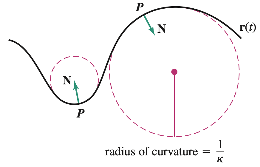
The radius is the reciprocal of the curvature:
\begin{equation*} R = \frac{1}{\kappa} = 2\sqrt{2} \end{equation*}
Step 2: Find the normal vector \(\v{N}\) To use the definition \(\v{N}(t) = \frac{\v{T}'(t)}{\|\v{T}'(t)\|}\text{,}\) we first need the general formula for \(\v{T}(t)\text{.}\)
\begin{align*} \|\v{r}'(t)\| \amp= \sqrt{1^2 + \left(\frac{1}{t}\right)^2} = \sqrt{\frac{t^2+1}{t^2}} = \frac{\sqrt{t^2+1}}{t} \end{align*}
Now we define \(\v{T}(t)\text{:}\)
\begin{align*} \v{T}(t) \amp= \frac{\v{r}'(t)}{\|\v{r}'(t)\|} = \frac{\la 1, t^{-1} \ra}{\frac{\sqrt{t^2+1}}{t}} = \frac{t}{\sqrt{t^2+1}} \la 1, t^{-1} \ra \\ \amp= \la \frac{t}{(t^2+1)^{1/2}}, \frac{1}{(t^2+1)^{1/2}} \ra \\ \amp= \la t(t^2+1)^{-1/2}, (t^2+1)^{-1/2} \ra \end{align*}
Next, we differentiate \(\v{T}(t)\) to find \(\v{T}'(t)\text{.}\)
\begin{align*} x_{\v{T}}'(t) \amp= (1)(t^2+1)^{-1/2} + t\left(-\frac{1}{2}\right)(t^2+1)^{-3/2}(2t) \\ \amp= (t^2+1)^{-1/2} - t^2(t^2+1)^{-3/2} \\ \amp= \frac{t^2+1}{(t^2+1)^{3/2}} - \frac{t^2}{(t^2+1)^{3/2}} = \frac{1}{(t^2+1)^{3/2}} \\ y_{\v{T}}'(t) \amp= -\frac{1}{2}(t^2+1)^{-3/2}(2t) = \frac{-t}{(t^2+1)^{3/2}} \end{align*}
Evaluating at \(t=1\text{:}\)
\begin{align*} \v{T}'(1) \amp= \la \frac{1}{(2)^{3/2}}, \frac{-1}{(2)^{3/2}} \ra = \la \frac{1}{2\sqrt{2}}, -\frac{1}{2\sqrt{2}} \ra = \frac{1}{2\sqrt{2}}\la 1, -1 \ra \end{align*}
Finally, we normalize this vector. Since \(\frac{1}{2\sqrt{2}}\) is just a scalar, the direction is clearly \(\la 1, -1 \ra\text{.}\)
\begin{align*} \v{N}(1) \amp= \frac{\v{T}'(1)}{\|\v{T}'(1)\|} = \frac{\la 1, -1 \ra}{\sqrt{1^2+(-1)^2}} = \frac{1}{\sqrt{2}}\la 1, -1 \ra \end{align*}
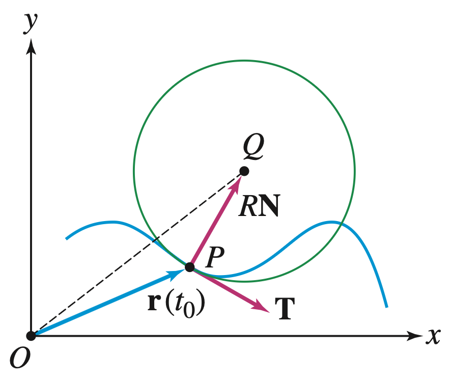
Step 3: Find the center \(Q\) We use the vector addition formula:
\begin{align*} \overrightarrow{OQ} \amp= \v{r}(1) + \frac{1}{\kappa} \v{N}(1) \\ \amp= \la 1, 0 \ra + (2\sqrt{2}) \left[ \frac{1}{\sqrt{2}}\la 1, -1 \ra \right] \\ \amp= \la 1, 0 \ra + 2\la 1, -1 \ra \\ \amp= \la 1+2, 0-2 \ra = \la 3, -2 \ra \end{align*}
The center is \((3, -2)\text{.}\)
Step 4: Determine the equation of the osculating circle Using the center \((3, -2)\) and radius \(R = 2\sqrt{2}\) (so \(R^2 = 8\)):
\begin{equation*} (x-3)^2 + (y+2)^2 = 8 \end{equation*}

Worksheet Assigned Problems for Section 13.4

The problems listed below are assigned to be included in your problem set portfolio. Note that a specific selection of these problems will also form the written homework assignments. I recommend working through all of them to ensure a solid grasp of the material. Reach out to Richard for help if you get stuck or have any questions.
The solutions will be posted after the written homework due dates. If you have any questions about your work, talk to Richard and he is happy to discuss the process with you.

13.4.3.

Calculate \(\v{r}'(t)\) and \(\v{T}(t)\) for \(\v{r}(t) = \la 3+4t, 3-5t, 9t \ra\text{,}\) and evaluate \(\v{T}(1)\text{.}\)
Solution.
First, we compute the derivative \(\v{r}'(t)\text{:}\)
\begin{equation*} \v{r}'(t) = \la 4, -5, 9 \ra \end{equation*}
Next, we find the magnitude of the velocity vector:
\begin{equation*} \|\v{r}'(t)\| = \sqrt{4^2 + (-5)^2 + 9^2} = \sqrt{16 + 25 + 81} = \sqrt{122} \end{equation*}
The unit tangent vector is the velocity vector divided by its speed:
\begin{equation*} \v{T}(t) = \frac{\v{r}'(t)}{\|\v{r}'(t)\|} = \frac{1}{\sqrt{122}} \la 4, -5, 9 \ra \end{equation*}
Since \(\v{T}(t)\) is constant, evaluating it at \(t=1\) yields the exact same vector:
\begin{equation*} \v{T}(1) = \la \frac{4}{\sqrt{122}}, -\frac{5}{\sqrt{122}}, \frac{9}{\sqrt{122}} \ra \end{equation*}

13.4.9.

Calculate the curvature function \(\kappa(t)\) of \(\v{r}(t) = \la 4t+1, 4t-3, 2t \ra\) using TheoremΒ 13.4.6.
Solution.
First, we find the first and second derivatives of \(\v{r}(t)\text{:}\)
\begin{align*} \v{r}'(t) \amp= \la 4, 4, 2 \ra \\ \v{r}''(t) \amp= \la 0, 0, 0 \ra \end{align*}
Using TheoremΒ 13.4.6, the curvature is:
\begin{equation*} \kappa(t) = \frac{\|\v{r}'(t) \times \v{r}''(t)\|}{\|\v{r}'(t)\|^3} \end{equation*}
Since \(\v{r}''(t) = \v{0}\text{,}\) the cross product \(\v{r}'(t) \times \v{r}''(t)\) is the zero vector \(\v{0}\text{.}\) Its magnitude is \(0\text{.}\) Thus, the curvature is:
\begin{equation*} \kappa(t) = \frac{0}{\|\v{r}'(t)\|^3} = 0 \end{equation*}
(This makes geometric sense, as the parametrization describes a straight line, which has zero curvature everywhere).

13.4.13.

Evaluate the curvature of the curve \(\v{r}(t) = \la \cos(t), \sin(t), t^2 \ra\) at the point where \(t=\frac{\pi}{2}\) using TheoremΒ 13.4.6.
Solution.
We first compute the velocity and acceleration vectors:
\begin{align*} \v{r}'(t) \amp= \la -\sin(t), \cos(t), 2t \ra \\ \v{r}''(t) \amp= \la -\cos(t), -\sin(t), 2 \ra \end{align*}
Evaluating these at \(t = \frac{\pi}{2}\text{:}\)
\begin{align*} \v{r}'\lp \frac{\pi}{2} \rp \amp= \la -1, 0, \pi \ra \\ \v{r}''\lp \frac{\pi}{2} \rp \amp= \la 0, -1, 2 \ra \end{align*}
Next, compute the cross product:
\begin{align*} \v{r}'\lp \frac{\pi}{2} \rp \times \v{r}''\lp \frac{\pi}{2} \rp \amp= \begin{vmatrix} \v{i} \amp \v{j} \amp \v{k} \\ -1 \amp 0 \amp \pi \\ 0 \amp -1 \amp 2 \end{vmatrix} \\ \amp= \la 0 - (-\pi), 0 - (-2), 1 - 0 \ra = \la \pi, 2, 1 \ra \end{align*}
Now, find the magnitudes:
\begin{align*} \left\|\v{r}'\lp \frac{\pi}{2} \rp \times \v{r}''\lp \frac{\pi}{2} \rp\right\| \amp= \sqrt{\pi^2 + 2^2 + 1^2} = \sqrt{\pi^2 + 5} \\ \left\|\v{r}'\lp \frac{\pi}{2} \rp\right\| \amp= \sqrt{(-1)^2 + 0^2 + \pi^2} = \sqrt{1 + \pi^2} \end{align*}
Using TheoremΒ 13.4.6, the curvature is:
\begin{equation*} \kappa\lp \frac{\pi}{2} \rp = \frac{\sqrt{\pi^2 + 5}}{\lp \sqrt{1 + \pi^2} \rp^3} = \frac{\sqrt{\pi^2 + 5}}{\lp 1 + \pi^2 \rp^{3/2}} \end{equation*}

13.4.17.

Find the curvature of the plane curve \(y = t^4\) at the point where \(t=2\text{.}\)
Solution.
We can treat this as a function \(f(t) = t^4\) and use the curvature formula for a graph from TheoremΒ 13.4.13:
\begin{equation*} \kappa(t) = \frac{|f''(t)|}{\lp 1 + \lp f'(t) \rp^2 \rp^\frac{3}{2}} \end{equation*}
Compute the derivatives:
\begin{align*} f'(t) \amp= 4t^3 \implies f'(2) = 4(8) = 32 \\ f''(t) \amp= 12t^2 \implies f''(2) = 12(4) = 48 \end{align*}
Substitute these values into the formula:
\begin{equation*} \kappa(2) = \frac{|48|}{\lp 1 + (32)^2 \rp^\frac{3}{2}} = \frac{48}{\lp 1 + 1024 \rp^\frac{3}{2}} = \frac{48}{1025^\frac{3}{2}} \end{equation*}

13.4.25.

Show that the curvature function of the parametrization \(\v{r}(t) = \la a\cos(t), b\sin(t) \ra \) of the ellipse \(\lp \dfrac{x}{a} \rp^2 + \lp \dfrac{y}{b} \rp^2 = 1\) is
\begin{equation*} \kappa(t) = \frac{ab}{\lp b^2\cos^2(t) + a^2\sin^2(t)\rp^\frac{3}{2}} \end{equation*}
Solution.
We use the curvature formula for a plane curve \(\v{r}(t) = \la x(t), y(t) \ra\text{:}\)
\begin{equation*} \kappa(t) = \frac{|x'(t)y''(t) - y'(t)x''(t)|}{\lp \lp x'(t)\rp^2 + \lp y'(t)\rp^2 \rp^\frac{3}{2}} \end{equation*}
Compute the first and second derivatives of the components:
\begin{align*} x(t) \amp= a\cos(t) \amp y(t) \amp= b\sin(t) \\ x'(t) \amp= -a\sin(t) \amp y'(t) \amp= b\cos(t) \\ x''(t) \amp= -a\cos(t) \amp y''(t) \amp= -b\sin(t) \end{align*}
Now, evaluate the numerator:
\begin{align*} x'(t)y''(t) - y'(t)x''(t) \amp= (-a\sin(t))(-b\sin(t)) - (b\cos(t))(-a\cos(t)) \\ \amp= ab\sin^2(t) + ab\cos^2(t) \\ \amp= ab\lp \sin^2(t) + \cos^2(t) \rp = ab \end{align*}
Evaluate the term inside the denominator:
\begin{equation*} \lp x'(t)\rp^2 + \lp y'(t)\rp^2 = (-a\sin(t))^2 + (b\cos(t))^2 = a^2\sin^2(t) + b^2\cos^2(t) \end{equation*}
Substitute these into the curvature formula (and note that \(a,b \gt 0\) typically for an ellipse, so \(|ab| = ab\)):
\begin{equation*} \kappa(t) = \frac{ab}{\lp a^2\sin^2(t) + b^2\cos^2(t) \rp^\frac{3}{2}} \end{equation*}
Since addition is commutative, we have verified the given formula.

13.4.31.

Compute the curvature of \(\la t\cos(t), \sin(t) \ra\) at the point where \(t=\pi\) using [insert formula].
Solution.
We use the curvature formula for a plane curve. First, find the derivatives:
\begin{align*} x(t) \amp= t\cos(t) \implies x'(t) = \cos(t) - t\sin(t) \\ x''(t) \amp= -\sin(t) - \lp \sin(t) + t\cos(t) \rp = -2\sin(t) - t\cos(t) \\ y(t) \amp= \sin(t) \implies y'(t) = \cos(t) \implies y''(t) = -\sin(t) \end{align*}
Evaluate these derivatives at \(t = \pi\text{:}\)
\begin{align*} x'(\pi) \amp= \cos(\pi) - \pi\sin(\pi) = -1 - 0 = -1 \\ x''(\pi) \amp= -2\sin(\pi) - \pi\cos(\pi) = 0 - \pi(-1) = \pi \\ y'(\pi) \amp= \cos(\pi) = -1 \\ y''(\pi) \amp= -\sin(\pi) = 0 \end{align*}
Substitute these into the curvature formula:
\begin{align*} \kappa(\pi) \amp= \frac{|x'(\pi)y''(\pi) - y'(\pi)x''(\pi)|}{\lp \lp x'(\pi)\rp^2 + \lp y'(\pi)\rp^2 \rp^\frac{3}{2}} \\ \amp= \frac{|(-1)(0) - (-1)(\pi)|}{\lp (-1)^2 + (-1)^2 \rp^\frac{3}{2}} \\ \amp= \frac{|\pi|}{\lp 2 \rp^\frac{3}{2}} = \frac{\pi}{2\sqrt{2}} \end{align*}

13.4.37.

Find the normal vector \(\v{N}(t)\) to \(\v{r} = \la 4, \sin(2t), \cos(2t) \ra\text{.}\)
Solution.
First, find the velocity vector and its magnitude:
\begin{align*} \v{r}'(t) \amp= \la 0, 2\cos(2t), -2\sin(2t) \ra \\ \|\v{r}'(t)\| \amp= \sqrt{0^2 + 4\cos^2(2t) + 4\sin^2(2t)} = \sqrt{4\lp \cos^2(2t) + \sin^2(2t) \rp} = \sqrt{4} = 2 \end{align*}
Next, find the unit tangent vector \(\v{T}(t)\text{:}\)
\begin{equation*} \v{T}(t) = \frac{\v{r}'(t)}{\|\v{r}'(t)\|} = \frac{1}{2} \la 0, 2\cos(2t), -2\sin(2t) \ra = \la 0, \cos(2t), -\sin(2t) \ra \end{equation*}
To find the normal vector \(\v{N}(t)\text{,}\) compute \(\v{T}'(t)\) and its magnitude:
\begin{align*} \v{T}'(t) \amp= \la 0, -2\sin(2t), -2\cos(2t) \ra \\ \|\v{T}'(t)\| \amp= \sqrt{0^2 + 4\sin^2(2t) + 4\cos^2(2t)} = \sqrt{4} = 2 \end{align*}
Finally, the normal vector is:
\begin{equation*} \v{N}(t) = \frac{\v{T}'(t)}{\|\v{T}'(t)\|} = \frac{1}{2} \la 0, -2\sin(2t), -2\cos(2t) \ra = \la 0, -\sin(2t), -\cos(2t) \ra \end{equation*}

13.4.39.

Find the normal vectors to \(\v{r}(t) = \la t, \cos(t) \ra\) at \(t = \dfrac{\pi}{4}\) and \(t = \dfrac{3\pi}{4}\text{.}\)
Solution.
The normal vector to \(\v{r}(t) = \la t, \cos(t) \ra\) is \(\v{T}'(t)\text{,}\) where \(\v{T}(t) = \frac{\v{r}'(t)}{\|\v{r}'(t)\|}\) is the unit tangent vector. We have
\begin{align*} \v{r}'(t) \amp= \la 1, -\sin(t) \ra \\ \|\v{r}'(t)\| \amp= \sqrt{1 + \sin^2(t)} \end{align*}
Hence,
\begin{equation*} \v{T}(t) = \frac{1}{\sqrt{1 + \sin^2(t)}}\la 1, -\sin(t) \ra \end{equation*}
We compute the derivative of \(\v{T}(t)\) to find the normal vector. We use the Product Rule and the Chain Rule to obtain
\begin{align*} \v{T}'(t) \amp= \frac{1}{\sqrt{1 + \sin^2(t)}} \frac{d}{dt} \la 1, -\sin(t) \ra + \lp \frac{1}{\sqrt{1 + \sin^2(t)}} \rp' \la 1, -\sin(t) \ra \\ \amp= \frac{1}{\sqrt{1 + \sin^2(t)}} \la 0, -\cos(t) \ra - \frac{1}{1 + \sin^2(t)} \cdot \frac{2\sin(t)\cos(t)}{2\sqrt{1 + \sin^2(t)}} \la 1, -\sin(t) \ra \\ \amp= \frac{1}{\sqrt{1 + \sin^2(t)}} \la 0,-\cos(t) \ra - \frac{\sin(2t)}{2\lp 1 + \sin^2(t) \rp^{3/2}} \la 1, -\sin(t) \ra \end{align*}
At \(t = \dfrac{\pi}{4}\text{,}\) we obtain the normal vector
\begin{align*} \v{T}'\lp \frac{\pi}{4} \rp \amp= \frac{1}{\sqrt{1 + \frac{1}{2}}} \la 0, -\frac{1}{\sqrt{2}} \ra - \frac{1}{2 \lp 1 + \frac{1}{2} \rp^{3/2}} \la 1, -\frac{1}{\sqrt{2}} \ra \\ \amp= \la 0, -\frac{1}{\sqrt{3}} \ra - \la \frac{\sqrt{2}}{3\sqrt{3}}, \frac{-1}{3\sqrt{3}} \ra \\ \amp= \la \frac{-\sqrt{2}}{3\sqrt{3}}, \frac{-2}{3\sqrt{3}} \ra \end{align*}
At \(t = \dfrac{3\pi}{4}\text{,}\) we obtain
\begin{align*} \v{T}'\lp \frac{3\pi}{4} \rp \amp= \frac{1}{\sqrt{1 + \frac{1}{2}}} \la 0, \frac{1}{\sqrt{2}} \ra - \frac{-1}{2 \lp 1 + \frac{1}{2} \rp^{3/2}} \la 1, -\frac{1}{\sqrt{2}} \ra \\ \amp= \la 0, \frac{1}{\sqrt{3}} \ra + \la \frac{\sqrt{2}}{3\sqrt{3}}, \frac{-1}{3\sqrt{3}} \ra \\ \amp= \la \frac{\sqrt{2}}{3\sqrt{3}}, \frac{2}{3\sqrt{3}} \ra \end{align*}

13.4.43.

Find \(\v{T}\text{,}\) \(\v{N}\text{,}\) and \(\v{B}\) for the curve \(\v{r}(t) = \la t,t^2,\dfrac{2}{3}t^3 \ra\) at the point \(\lp 1,1,\dfrac{2}{3} \rp\text{.}\)
Hint.
After finding \(\v{T}'\text{,}\) plug in the specific value for \(t\) before computing \(\v{N}\) and \(\v{B}\text{.}\)
Solution.
The point \(\lp 1, 1, \frac{2}{3} \rp\) corresponds to \(t=1\text{.}\) Let’s find the derivatives and speed.
\begin{align*} \v{r}'(t) \amp= \la 1, 2t, 2t^2 \ra \\ v(t) \amp= \sqrt{1 + 4t^2 + 4t^4} = \sqrt{(1+2t^2)^2} = 1+2t^2 \end{align*}
Unit Tangent Vector \(\v{T}\text{:}\)
\begin{align*} \v{T}(t) \amp= \frac{\v{r}'(t)}{v(t)} = \la \frac{1}{1+2t^2}, \frac{2t}{1+2t^2}, \frac{2t^2}{1+2t^2} \ra \\ \v{T}(1) \amp= \la \frac{1}{3}, \frac{2}{3}, \frac{2}{3} \ra \end{align*}
Normal Vector \(\v{N}\text{:}\) We differentiate each component of \(\v{T}(t)\) using the Quotient Rule:
\begin{align*} x_{\v{T}}'(t) \amp= \frac{0 - 1(4t)}{(1+2t^2)^2} = \frac{-4t}{(1+2t^2)^2} \\ y_{\v{T}}'(t) \amp= \frac{2(1+2t^2) - 2t(4t)}{(1+2t^2)^2} = \frac{2 - 4t^2}{(1+2t^2)^2} \\ z_{\v{T}}'(t) \amp= \frac{4t(1+2t^2) - 2t^2(4t)}{(1+2t^2)^2} = \frac{4t}{(1+2t^2)^2} \end{align*}
Evaluate at \(t=1\text{:}\)
\begin{align*} \v{T}'(1) \amp= \la \frac{-4}{9}, \frac{-2}{9}, \frac{4}{9} \ra \\ \|\v{T}'(1)\| \amp= \sqrt{\frac{16}{81} + \frac{4}{81} + \frac{16}{81}} = \sqrt{\frac{36}{81}} = \frac{6}{9} = \frac{2}{3} \end{align*}
Normalize to find \(\v{N}(1)\text{:}\)
\begin{equation*} \v{N}(1) = \frac{3}{2} \la -\frac{4}{9}, -\frac{2}{9}, \frac{4}{9} \ra = \la -\frac{2}{3}, -\frac{1}{3}, \frac{2}{3} \ra \end{equation*}
Binormal Vector \(\v{B}\text{:}\)
\begin{align*} \v{B}(1) \amp= \v{T}(1) \times \v{N}(1) = \begin{vmatrix} \v{i} \amp \v{j} \amp \v{k} \\ 1/3 \amp 2/3 \amp 2/3 \\ -2/3 \amp -1/3 \amp 2/3 \end{vmatrix} \\ \amp= \frac{1}{9} \begin{vmatrix} \v{i} \amp \v{j} \amp \v{k} \\ 1 \amp 2 \amp 2 \\ -2 \amp -1 \amp 2 \end{vmatrix} = \frac{1}{9} \la 4 - (-2), -(2 - (-4)), -1 - (-4) \ra \\ \amp= \frac{1}{9} \la 6, -6, 3 \ra = \la \frac{2}{3}, -\frac{2}{3}, \frac{1}{3} \ra \end{align*}

13.4.49.

Find \(\v{N}\) for the curve \(\la \dfrac{t^2}{2}, \dfrac{t^3}{3}, t \ra\) at the point where \(t=1\) using the formula
\begin{equation*} \v{N}(t) = \frac{v(t)\v{r}''(t) - v'(t)\v{r}'(t)}{\|v(t)\v{r}''(t) - v'(t)\v{r}'(t)\|} \end{equation*}
where \(v(t) = \|\v{r}'(t) \|\text{.}\)
Solution.
First compute the velocity and acceleration vectors, and the speed:
\begin{align*} \v{r}'(t) \amp= \la t, t^2, 1 \ra \implies \v{r}'(1) = \la 1, 1, 1 \ra \\ \v{r}''(t) \amp= \la 1, 2t, 0 \ra \implies \v{r}''(1) = \la 1, 2, 0 \ra \\ v(t) \amp= \|\v{r}'(t)\| = \sqrt{t^2 + t^4 + 1} \implies v(1) = \sqrt{3} \\ v'(t) \amp= \frac{2t + 4t^3}{2\sqrt{t^2+t^4+1}} = \frac{t + 2t^3}{\sqrt{t^2+t^4+1}} \implies v'(1) = \frac{3}{\sqrt{3}} = \sqrt{3} \end{align*}
Now compute the unnormalized vector \(\v{u} = v(1)\v{r}''(1) - v'(1)\v{r}'(1)\text{:}\)
\begin{align*} \v{u} \amp= \sqrt{3} \la 1, 2, 0 \ra - \sqrt{3} \la 1, 1, 1 \ra \\ \amp= \la \sqrt{3} - \sqrt{3}, 2\sqrt{3} - \sqrt{3}, 0 - \sqrt{3} \ra = \la 0, \sqrt{3}, -\sqrt{3} \ra = \sqrt{3}\la 0, 1, -1 \ra \end{align*}
Find the magnitude and normalize to get \(\v{N}\text{:}\)
\begin{align*} \|\v{u}\| \amp= \sqrt{3}\sqrt{0^2 + 1^2 + (-1)^2} = \sqrt{3}\sqrt{2} = \sqrt{6} \\ \v{N}(1) \amp= \frac{\sqrt{3}\la 0, 1, -1 \ra}{\sqrt{6}} = \frac{1}{\sqrt{2}} \la 0, 1, -1 \ra = \la 0, \frac{1}{\sqrt{2}}, -\frac{1}{\sqrt{2}} \ra \end{align*}

13.4.55.

Let \(\v{r}(t) = \la t,1-t,t^2 \ra\text{.}\)
  1. Find the general formulas for \(\v{T}\) and \(\v{N}\) as functions of \(t\text{.}\)
  2. Find the general formula for \(\v{B}\) as a function of \(t\text{.}\)
  3. What can you conclude about the osculating planes of the curve based on your answer to (b)?
Solution.
  1. Differentiating gives \(\v{r}'(t) = \la 1, -1, 2t \ra\text{,}\) so that
    \begin{align*} \v{T}(t) \amp= \frac{\v{r}'(t)}{\|\v{r}'(t)\|} \\ \amp= \frac{1}{\sqrt{1^2 + (-1)^2 + (2t)^2}} \la 1, -1, 2t \ra \\ \amp= \left\langle \frac{1}{\sqrt{4t^2+2}}, -\frac{1}{\sqrt{4t^2+2}}, \frac{2t}{\sqrt{4t^2+2}} \right\rangle \end{align*}
    The derivatives of the components of \(\v{T}(t)\) are
    \begin{align*} \frac{d}{dt} \lp \frac{1}{\sqrt{4t^2+2}} \rp \amp= -\frac{4t}{(4t^2+2)^{3/2}} \\ \frac{d}{dt} \lp -\frac{1}{\sqrt{4t^2+2}} \rp \amp= \frac{4t}{(4t^2+2)^{3/2}} \\ \frac{d}{dt} \lp \frac{2t}{\sqrt{4t^2+2}} \rp \amp= \frac{(4t^2+2)^{1/2}(2) - 2t \cdot \frac{1}{2}(4t^2+2)^{-1/2} \cdot 8t}{4t^2+2} \\ \amp= \frac{2(4t^2+2) - 8t^2}{(4t^2+2)^{3/2}} = \frac{4}{(4t^2+2)^{3/2}} \end{align*}
    Thus,
    \begin{align*} \v{T}'(t) \amp= \left\langle -\frac{4t}{(4t^2+2)^{3/2}}, \frac{4t}{(4t^2+2)^{3/2}}, \frac{4}{(4t^2+2)^{3/2}} \right\rangle \\ \amp= \frac{1}{(4t^2+2)^{3/2}} \la -4t, 4t, 4 \ra \end{align*}
    To find \(\v{N}(t)\) we must find \(\|\v{T}'(t)\|\text{:}\)
    \begin{align*} \|\v{T}'(t)\| \amp= \frac{1}{(4t^2+2)^{3/2}} \sqrt{(-4t)^2 + (4t)^2 + 4^2} \\ \amp= \frac{1}{(4t^2+2)^{3/2}} \sqrt{32t^2+16} \\ \amp= \frac{\sqrt{8}\sqrt{4t^2+2}}{(4t^2+2)^{3/2}} = \frac{\sqrt{8}}{4t^2+2} \end{align*}
    So
    \begin{align*} \v{N}(t) \amp= \frac{\v{T}'(t)}{\|\v{T}'(t)\|} = \frac{\frac{1}{(4t^2+2)^{3/2}} \la -4t, 4t, 4 \ra}{\frac{\sqrt{8}}{4t^2+2}} \\ \amp= \frac{4t^2+2}{(4t^2+2)^{3/2}\sqrt{8}} \la -4t, 4t, 4 \ra \\ \amp= \frac{1}{\sqrt{4t^2+2}\sqrt{8}} \la -4t, 4t, 4 \ra \\ \amp= \frac{1}{\sqrt{32t^2+16}} \la -4t, 4t, 4 \ra \\ \amp= \frac{1}{\sqrt{16(2t^2+1)}} 4 \la -t, t, 1 \ra \\ \amp= \frac{1}{4\sqrt{2t^2+1}} 4 \la -t, t, 1 \ra = \frac{1}{\sqrt{2t^2+1}} \la -t, t, 1 \ra \end{align*}
  2. Using the cross product formula \(\v{B}(t) = \v{T}(t) \times \v{N}(t)\text{:}\)
    \begin{align*} \v{B}(t) \amp= \lp \frac{1}{\sqrt{4t^2+2}} \rp \lp \frac{1}{\sqrt{2t^2+1}} \rp \begin{vmatrix} \v{i} \amp \v{j} \amp \v{k} \\ 1 \amp -1 \amp 2t \\ -t \amp t \amp 1 \end{vmatrix} \\ \amp= \frac{1}{\sqrt{2}\sqrt{2t^2+1}\sqrt{2t^2+1}} \la -1-2t^2, -(1-(-2t^2)), t-t \ra \\ \amp= \frac{1}{\sqrt{2}(2t^2+1)} \la -(1+2t^2), -(1+2t^2), 0 \ra \\ \amp= \frac{-(1+2t^2)}{\sqrt{2}(1+2t^2)} \la 1, 1, 0 \ra \\ \amp= \left\langle -\frac{1}{\sqrt{2}}, -\frac{1}{\sqrt{2}}, 0 \right\rangle \end{align*}
  3. Since the binormal vector \(\v{B}(t) = \la -\frac{1}{\sqrt{2}}, -\frac{1}{\sqrt{2}}, 0 \ra\) is constant, the normal vector to the osculating plane never changes. Therefore, the osculating plane is the same for all \(t\text{.}\) All osculating planes are the fixed plane \(x + y = 1\text{.}\)

13.4.67.

Find an equation of the osculating circle to the curve \(\v{r}(t) = \la 1-\sin(t), 1-2\cos(t) \ra\) at the point where \(t=\pi\) or indicate that none exists.
Solution.
Step 1: Compute derivatives at \(t=\pi\)
\begin{align*} \v{r}(\pi) \amp= \la 1-\sin(\pi), 1-2\cos(\pi) \ra = \la 1, 3 \ra \\ \v{r}'(t) \amp= \la -\cos(t), 2\sin(t) \ra \implies \v{r}'(\pi) = \la 1, 0 \ra \\ \v{r}''(t) \amp= \la \sin(t), 2\cos(t) \ra \implies \v{r}''((\pi) = \la 0, -2 \ra \end{align*}
Step 2: Find the radius of curvature
\begin{align*} \kappa(\pi) \amp= \frac{|x'y'' - y'x''|}{\lp (x')^2 + (y')^2 \rp^{3/2}} = \frac{|(1)(-2) - (0)(0)|}{\lp 1^2 + 0^2 \rp^{3/2}} = 2 \\ R \amp= \frac{1}{\kappa(\pi)} = \frac{1}{2} \end{align*}
Step 3: Find the Normal Vector Since the velocity vector is \(\v{r}'(\pi) = \la 1, 0 \ra\text{,}\) the unit tangent vector is \(\v{T}(\pi) = \la 1, 0 \ra\text{.}\) In 2D, the principal normal vector \(\v{N}\) is orthogonal to \(\v{T}\) and points in the direction the curve is bending (concave side). Since the acceleration is \(\v{r}''(\pi) = \la 0, -2 \ra\text{,}\) the curve is bending downwards. Thus:
\begin{equation*} \v{N}(\pi) = \la 0, -1 \ra \end{equation*}
Step 4: Find the Center and Equation The center \(Q\) is found by translating from the point \(P(1,3)\) along the normal vector by the distance \(R\text{:}\)
\begin{equation*} \overrightarrow{OQ} = \v{r}(\pi) + R\v{N}(\pi) = \la 1, 3 \ra + \frac{1}{2}\la 0, -1 \ra = \la 1, \frac{5}{2} \ra \end{equation*}
With center \(\lp 1, \frac{5}{2} \rp\) and radius \(R = \frac{1}{2}\text{,}\) the equation of the osculating circle is:
\begin{equation*} (x - 1)^2 + \lp y - \frac{5}{2} \rp^2 = \frac{1}{4} \end{equation*}