
Section 15.1 Integration in Two Variables

In single-variable calculus, we discovered that the definite integral of a function \(f(x)\) over an interval \([a,b]\) represents the "net area" between the curve and the \(x\)-axis. By partitioning the interval into smaller sub-intervals, we summed up the areas of infinitely many rectangles to arrive at a precise value.
In this section, we extend this idea to functions of two variables, \(z = f(x,y)\text{.}\) Instead of finding the area under a curve, we are now interested in finding the volume of a solid under a surface. We will begin by defining the double integral over a rectangular region as a limit of Riemann sums, conceptually similar to the "french fries" model, where we sum up the volumes of skinny rectangular boxes.
We will also explore Fubini’s Theorem, which provides a practical way to evaluate these volumes by "slicing" the solid and integrating one variable at a time. This transformation into iterated integrals allows us to use all the integration techniques we mastered in previous terms to solve complex 3D problems.
Recall back in MTH 252Z (or MTH 252), we can find the area of a region under a curve in \(\R^2\) by integrating the single-variable function. Similarly, if we boost everything up a dimension, then we should be able to find the volume of a solid in \(\R^3\) by integrating the function of two variables.
If we remember how we defined the integral of a single-variable function back in MTH 252Z (or MTH 252), then we can use the same idea to define the integral of a function of two variables.

Subsection Review: Integration and Riemann Sum in \(\R^2\)

Recall back in MTH 252Z (or MTH 252), we defined the integral of a function as the limit of Riemann sums. More specifically, we can partition the region of interest under the curve into a bunch of skinny rectangles, and we can estimate the area of the region by summing up the areas of the rectangles. This process is called a Riemann Sum.
Figure 15.1.1. Riemann Sum in \(\R^2\)
Mathematically speaking, if we have a function \(y = f(x)\) defined on the interval \([a,b]\text{.}\) Then we can partition the interval \([a,b]\) into \(N\) sub-intervals
\begin{equation*} P: \, a = x_0 \lt x_1 \lt x_2 \lt \cdots \lt x_N = b \end{equation*}
The difference between two consecutive points in the partition, \(\Delta x\text{,}\) is the width of the rectangles.
In each sub-interval \([x_i, x_{i + 1}]\text{,}\) we can choose a sample point within the sub-interval to determine the height of the rectangle
\begin{equation*} C = \left\{c_1, c_2, \ldots, c_N\right\} \, , \qquad c_i \in [x_i, x_{i + 1}] \end{equation*}
The function value at the sample point, \(f(c_i)\text{,}\) is the height of the rectangle.
Putting these two pieces together, we can estimate the area of the region under the curve by summing up the areas of the rectangles as follows:
\begin{equation*} A \approx \sum_{i = 1}^N f(c_i) \Delta x \end{equation*}
Recall that the area of all rectangles summing up together will be closer and closer to the actual area of the region as we make the partition finer and finer, using more and more rectangles. That is, our Riemann sum estimate will get better and better as we increase the number of rectangles. Using calculus language, the limit of the Riemann sum as the number of rectangles goes to infinity is the actual area of the region under the curve. Symbolically, we can write this as
\begin{equation*} A = \lim_{N \to \infty} \sum_{i = 1}^N f(c_i) \Delta x \end{equation*}
This is how we defined the definite integral of a single-variable function back in MTH 252Z (or MTH 252).
\begin{equation*} \int _a^b f(x)\, dx := \lim_{N \to \infty} \sum_{i = 1}^N f(c_i) \Delta x \end{equation*}
If we break down each component of the definite integral and match up the notation, we know that
  • the definite sign, \(\int\text{,}\) means summation (a cursive S).
  • \(f(x)\) is the function value at some random point \(x\text{,}\) which works like the height of the representative rectangle. This is also called the integrand.
  • \(dx\) is the width of the representative rectangle (\(dx\) means \(\Delta x\) when the change is really really really small). This is also called the differential.
  • the \(a\) and the \(b\) tells us about the interval. They are called the limits of integration. \(a\) is the lower limit and \(b\) is the upper limit.
Now that we have reviewed what integration means (summing up a bunch of stuff), we can now extend this idea to functions of two variables!
P.S.: if you need a more detailed review, here is Richard’s MTH 252Z note on Approximating Area Using Riemann Sums, Definite Integrals, and Definite Integrals as Summing Up Pieces last term (Fall 2025).

Subsection Volume of a Solid

Now let’s boost everything up a dimension! In a nutshell, we can find the volume of a solid by doing something like the image below:
Figure 15.1.2. Riemann Sum in \(\R^3\) using french fries
Now let’s get into the details! Rather than working with a single-variable function, we will now work with a function of two variables. Let’s call this function \(z = f(x,y)\text{.}\) The graph of \(f\) is a surface in \(\R^3\text{,}\) and the "region" under the surface is now a solid!
Figure 15.1.3. "Region" under the surface \(z = f(x,y)\) on \([a,b] \times [c,d]\) is a solid.
Observe from the diagram above that we can determine the solid by looking at the surface over a region on the \(xy\)-plane. Usually, we can describe the region of interest on the \(xy\)-plane by
\begin{equation*} \c{R} = [a,b] \times [c,d] = \left\{(x,y)\in \R^2 \mid a \leq x \leq b\, , \quad c \leq y \leq d\right\} \end{equation*}
The region \(\c{R}\) in the diagram is a rectangle.
If we want to apply the Riemann sum idea to partitioning and finding sample points here, we will need to do it in two dimensions: along the \(x\)-axis and along the \(y\)-axis. This will give us a bunch of tiny sub-rectangles within the region, and we can pick a point within each sub-rectangle to be the sample point.
Figure 15.1.4. Partitioning the region \(\c{R}\) into sub-rectangles.
Now let’s think about how to find the volume of the solid! For each of the sub-rectangle, we can construct a skinny rectangular box that has the same base as the sub-rectangle and the height equal to the function value at the sample point. Then the volume of the skinny rectangular box is \(f\lp x_{ij}^*, y_{ij}^* \rp\, \Delta A\) (base times height), where \(\Delta A\) is the area of the sub-rectangle and \((x_{ij}^*, y_{ij}^*)\) is the sample point in the sub-rectangle. To find the total volume of the solid, we will just need to sum up the volumes of all the skinny rectangular boxes. Symbolically, we can write this as
\begin{equation*} V \approx S_{N, M} = \sum_{i = 1}^N \sum_{j = 1}^M f\lp x_{ij}^*, y_{ij}^* \rp\, \Delta A \end{equation*}
where \(N\) and \(M\) are the number of partitions along the \(x\)-axis and the \(y\)-axis, respectively, and \(S_{N,M}\) is the Riemann sum estimate of the volume of the solid using \(N\) and \(M\) partitions.
Figure 15.1.5. Partitioning the solid into skinny rectangular boxes.
As you can imagine, the more and more skinny rectangular boxes we have, the better and better our estimate of the volume will be. Using calculus language, the limit of the Riemann sum as the number of boxes goes to infinity is the actual volume of the solid. Symbolically, we can write this as
\begin{equation*} V = \lim_{N,M \to \infty} \sum_{i = 1}^N \sum_{j = 1}^M f\lp x_{ij}^*, y_{ij}^* \rp\, \Delta A \end{equation*}
Observe that there are two summation notations in the expression above, then we will need two integration signs to capture the idea of summing up in two dimensions. This is how we define the double integral of a function of two variables over a rectangular region to find the volume of the solid under the surface.

Definition 15.1.6. Double Integral over a Rectangular Region.

The double integral of \(f(x,y)\) over a rectangular region \(\c{R}\) is defined as the limit
\begin{equation*} \iint_\c{R} f(x,y)\, dA = \lim_{N,M \to \infty} \sum_{i = 1}^N \sum_{j = 1}^M f\lp x_{ij}^*, y_{ij}^* \rp\, \Delta A \end{equation*}
If the limit exists, we say that \(f(x,y)\) is integrable over \(\c{R}\text{.}\)

Note 15.1.7. But Richard... Do all the sub-rectangles have to be the same size?

The short answer is no. The only thing we want to make sure is to let the area of each sub-rectangle go to zero.
But there is a false equivalence of "having infinite number of sub-rectangles" and "having all the sub-rectangles to have the area approaching zero". It is totally possible to have infinitely many sub-rectangles but the area of some of the sub-rectangles does not approach zero. An easiest example is to split the rectangular region in half, and only partition one half into infinitely many sub-rectangles while leaving the other half as one big rectangle.
If we demand all the sub-rectangles to have the same area, then we can guarantee that the area of each sub-rectangle approaches zero as the number of sub-rectangles goes to infinity. Also, it is easier to find the area of each sub-rectangle if they are all the same size. Because of this convenience, we call this type of partition a regular partition.
If you relax this condition a bit and don’t require all the sub-rectangles to have the same area, then you can still do the Riemann sum by requiring the largest sub-rectangle to have the area approaching zero. This is how your textbook defines the Riemann sum.

Example 15.1.8.

Estimate the volume of the solid under the elliptic paraboloid \(z = 16 - x^2 - 2y^2\) over the region \([0,2] \times [0,2]\) using four sub-rectangles and the upper-right vertices of the sub-rectangles as sample points.
Hint.
The goal here is to estimate the volume of the solid under the surface using four rectangular boxes, as demonstrated in the figure below.
Figure 15.1.9. Graph of the surface \(f(x,y) = 16 - x^2 - 2y^2\) with four rectangular boxes estimating the volume using upper right vertices.
Graphically speaking, we can determine the coordinates of the upper-right vertices of the sub-rectangles, as demonstrated in the figure below.
Figure 15.1.10.
So how do we find the volume of each rectangular box?
Solution.
First, we need to set up the partition. The region \(\c{R}\) is a \([0,2] \times [0,2]\) square on the \(xy\)-plane. Dividing it into four equal sub-rectangles gives a \(2 \times 2\) grid.
The width and length of each sub-rectangle are \(\Delta x = \frac{2-0}{2} = 1\) and \(\Delta y = \frac{2-0}{2} = 1\text{.}\) The area of each base is \(\Delta A = 1 \cdot 1 = 1\text{.}\)
Next, we identify the sample points. We are using the upper-right vertices for our \((x_{ij}^*, y_{ij}^*)\text{.}\) For the four sub-rectangles, these points are:
Now we calculate the heights by evaluating \(f(x,y) = 16 - x^2 - 2y^2\) at each sample point:
Finally, we sum the volumes of the four rectangular boxes:
\begin{align*} V \amp \approx \sum_{i=1}^2 \sum_{j=1}^2 f(x_{ij}^*, y_{ij}^*)\Delta A \\ \amp = (13 + 10 + 7 + 4)(1) \\ \amp = 34 \end{align*}
Just like when you first learned about integrals back in MTH 252Z (or MTH 252), we can sometimes find the value of the double integral using geometry if the solid has a nice shape that we know the volume formula for.

Example 15.1.11.

Evaluate the double integral \(\ds \iint_\c{R} \sqrt{1 - x^2}\, dA\text{,}\) where \(\c{R} = [-1,1] \times [-2,2]\text{.}\)
Solution.
Instead of finding an antiderivative, let’s look at the surface \(z = \sqrt{1 - x^2}\text{.}\) Squaring both sides gives \(z^2 = 1 - x^2\text{,}\) or \(x^2 + z^2 = 1\text{.}\) In \(\R^3\text{,}\) this represents a cylinder of radius 1 centered along the \(y\)-axis. Since \(z \geq 0\text{,}\) we are only looking at the top half of this cylinder.
Richard coded the surface and the region of interest below for you to visualize what the solid looks like.
Figure 15.1.12.
The region \(\c{R} = [-1,1] \times [-2,2]\) tells us that \(x\) goes from \(-1\) to \(1\) (which exactly matches the diameter of our cylinder) and \(y\) goes from \(-2\) to \(2\text{.}\)
Therefore, the solid is a half-cylinder with a length of \(4\) (since \(2 - (-2) = 4\)) and a semi-circular cross-section of radius 1. We can calculate the volume using basic geometry:
\begin{align*} \text{Area of base} \amp = \frac{1}{2}\pi r^2 = \frac{1}{2}\pi (1)^2 = \frac{\pi}{2} \\ \text{Volume} \amp = \text{Area} \cdot \text{length} = \frac{\pi}{2} \cdot 4 = 2\pi \end{align*}
So, \(\ds \iint_\c{R} \sqrt{1 - x^2}\, dA = 2\pi\text{.}\)

Subsection Iterated Integrals

In practice, we usually don’t have a nice shape that we can find the volume using geometry, so we will need to evaluate the double integral using calculus. One way to do so is to think about the double integral as an iterated integral, which takes in the following form
\begin{equation*} \iint_R f(x,y)\, dA = \int_a^b \int_c^d f(x,y)\, dy\, dx = \int_a^b \lp \int_c^d f(x,y)\, dy \rp \, dx \end{equation*}
Well this form makes sense. If the rectangular region \(\c{R}\) is \([a,b] \times [c,d]\text{,}\) then we can first fix the \(x\)-value and integrate with respect to \(y\) from \(c\) to \(d\text{.}\) This gives us the area of the cross-section of the solid at that particular \(x\)-value. Then we can integrate with respect to \(x\) from \(a\) to \(b\) to sum up all the cross-sectional areas to get the total volume of the solid (this is a similar idea to the Disk Method you learned back in MTH 252Z (or MTH 252)). The term "iterated integral" just means that we are integrating in succession.
Figure 15.1.13. The inner integral finds the cross-sectional area and the outer integral sums all cross-sectional areas to get the total volume.
There are two steps to evaluate a double integral using iterated integrals: evaluate the inner integral with respect to one variable first, treating the other variable as a constant, and then evaluate the outer integral with respect to the other variable. Now that we only deal with one variable for each integral, we can now use all the fun integral techniques you learned back in MTH 252Z (or MTH 252) to evaluate the inner and outer integrals!

Example 15.1.14.

Evaluate the double integral \(\ds \int_1^3 \int_0^\frac{\pi}{2} x\sin(y)\, dy\, dx\)
Solution.
We start by evaluating the inner integral with respect to \(y\text{,}\) treating \(x\) as a constant:
\begin{align*} \int_0^{\frac{\pi}{2}} x\sin(y)\, dy \amp = x \Big[ -\cos(y) \Big]_0^{\frac{\pi}{2}} \\ \amp = x \left( -\cos\left(\frac{\pi}{2}\right) - (-\cos(0)) \right) \\ \amp = x(0 + 1) = x \end{align*}
Next, we substitute this result into the outer integral and integrate with respect to \(x\text{:}\)
\begin{align*} \int_1^3 x\, dx \amp = \left[ \frac{1}{2}x^2 \right]_1^3 \\ \amp = \frac{9}{2} - \frac{1}{2} = 4 \end{align*}

Example 15.1.15.

Evaluate the double integral \(\ds \int_0^1 \int_0^1 \sqrt{x + y}\, dx\, dy\)
Solution.
We start by evaluating the inner integral with respect to \(x\text{,}\) treating \(y\) as a constant.
\begin{align*} \int_0^1 (x + y)^{1/2}\, dx \amp = \left[ \frac{2}{3}(x + y)^{3/2} \right]_{x=0}^{x=1} \\ \amp = \frac{2}{3} \big( (1 + y)^{3/2} - (0 + y)^{3/2} \big) \\ \amp = \frac{2}{3} \big( (y + 1)^{3/2} - y^{3/2} \big) \end{align*}
Now, we substitute this result back into the outer integral to integrate with respect to \(y\text{.}\)
\begin{gather*} \int_0^1 \frac{2}{3} \big( (y + 1)^{3/2} - y^{3/2} \big)\, dy \end{gather*}
We can evaluate this by integrating each term directly using the power rule.
\begin{align*} \amp \frac{2}{3} \left[ \frac{2}{5}(y + 1)^{5/2} - \frac{2}{5}y^{5/2} \right]_{y=0}^{y=1} \\ \amp = \frac{4}{15} \Big[ (y + 1)^{5/2} - y^{5/2} \Big]_0^1 \end{align*}
Next, we evaluate these terms at the boundaries \(y = 1\) and \(y = 0\text{.}\)
\begin{align*} \amp \frac{4}{15} \Big( \big( (1 + 1)^{5/2} - 1^{5/2} \big) - \big( (0 + 1)^{5/2} - 0^{5/2} \big) \Big) \\ \amp = \frac{4}{15} \Big( (2^{5/2} - 1) - (1 - 0) \Big) \end{align*}
Finally, we simplify the expression. Recognizing that \(2^{5/2} = (\sqrt{2})^5 = 4\sqrt{2}\text{,}\) we get our final exact answer.
\begin{align*} \frac{4}{15} \big( 4\sqrt{2} - 1 - 1 \big) \amp = \frac{4}{15} \big( 4\sqrt{2} - 2 \big) \\ \amp = \frac{16\sqrt{2} - 8}{15} \end{align*}

Example 15.1.16.

Evaluate the double integral \(\ds \iint_\c{R} \lp 6 - 2x - y \rp\, dA\text{,}\) where \(\c{R} = [0,1] \times [0,2]\text{.}\)
Hint.
There are two options here... We can integrate with respect to \(y\) first, then \(x\text{,}\) or we can integrate with respect to \(x\) first, then \(y\text{.}\) But which one will work out?
Let’s try them both out and see what happens!
Solution 1. If we integrate with respect to \(y\) first, then \(x\)
Let’s choose to integrate with respect to \(y\) first, then \(x\text{.}\)
Evaluating the inner integral with respect to \(y\text{:}\)
\begin{align*} \int_0^2 (6 - 2x - y)\, dy \amp = \left[ 6y - 2xy - \frac{1}{2}y^2 \right]_0^2 \\ \amp = \left( 12 - 4x - 2 \right) - (0) \\ \amp = 10 - 4x \end{align*}
Now, evaluating the outer integral with respect to \(x\text{:}\)
\begin{align*} \int_0^1 (10 - 4x)\, dx \amp = \left[ 10x - 2x^2 \right]_0^1 \\ \amp = 10 - 2 = 8 \end{align*}
Solution 2. If we integrate with respect to \(x\) first, then \(y\)
Evaluating the inner integral with respect to \(x\) (treating \(y\) as a constant):
\begin{align*} \int_0^1 (6 - 2x - y)\, dx \amp = \left[ 6x - x^2 - xy \right]_{x=0}^{x=1} \\ \amp = \left( 6(1) - (1)^2 - (1)y \right) - (0) \\ \amp = 6 - 1 - y \\ \amp = 5 - y \end{align*}
Now, evaluating the outer integral with respect to \(y\text{:}\)
\begin{align*} \int_0^2 (5 - y)\, dy \amp = \left[ 5y - \frac{1}{2}y^2 \right]_{y=0}^{y=2} \\ \amp = \left( 5(2) - \frac{1}{2}(2)^2 \right) - (0) \\ \amp = 10 - 2 = 8 \end{align*}
In the last example, we see that the answer of the double integral is the same regardless of the order in which the integration is performed (integrating with respect to \(y\) first or integrating with respect to \(x\) first). This is a special property of double integrals called Fubini’s Theorem. It is also the Fubini’s Theorem that allows us to evaluate the double integral as an iterated integral.
The proof of the Fubini’s Theorem is a bit technical. Intuitively, the volume of the solid should stay the same regardless of how we slice it up and sum up the pieces, as indicated in the following diagram.
Figure 15.1.18.
By the Fubini’s Theorem, we can choose the order of integration that makes the work easier.

Example 15.1.19.

Evaluate the double integral \(\ds \iint_\c{R} ye^{xy}\, dA\text{,}\) where \(\c{R} = [0,1] \times [0,\ln(2)]\text{.}\)
Solution.
We must choose the order of integration: \(dx\,dy\) or \(dy\,dx\text{.}\)
If we integrate with respect to \(y\) first, we have to evaluate \(\int ye^{xy}\, dy\text{,}\) which requires Integration by Parts. However, if we integrate with respect to \(x\) first, \(y\) is treated as a constant, and \(\int ye^{xy}\, dx = e^{xy}\text{,}\) which is much simpler. Therefore, we will use the order \(dx\,dy\text{.}\)
Setting up the iterated integral and evaluating the inner integral with respect to \(x\text{:}\)
\begin{align*} \int_0^{\ln(2)} \int_0^1 ye^{xy}\, dx\, dy \amp = \int_0^{\ln(2)} \Big[ e^{xy} \Big]_{x=0}^{x=1}\, dy \\ \amp = \int_0^{\ln(2)} (e^y - e^0)\, dy \\ \amp = \int_0^{\ln(2)} (e^y - 1)\, dy \end{align*}
Now, evaluate the outer integral with respect to \(y\text{:}\)
\begin{align*} \int_0^{\ln(2)} (e^y - 1)\, dy \amp = \Big[ e^y - y \Big]_0^{\ln(2)} \\ \amp = (e^{\ln(2)} - \ln(2)) - (e^0 - 0) \\ \amp = 2 - \ln(2) - 1 \\ \amp = 1 - \ln(2) \end{align*}
But be careful! When interchanging the order of integration, you will also need to change the limits of integration accordingly! In this section, we can just simply swap the limits of integration because the region is a rectangle (so the values of \(x\) and \(y\) are independent of each other). However, in the next section, we will investigate the double integrals over a more general region, which may require more work to change and adjust (and maybe even finding) the limits of integration when changing the order of integration.

Worksheet Assigned Problems for Section 15.1

The problems listed below are assigned to be included in your problem set portfolio. Note that a specific selection of these problems will also form the written homework assignments. I recommend working through all of them to ensure a solid grasp of the material. Reach out to Richard for help if you get stuck or have any questions.
The solutions will be posted after the written homework due dates. If you have any questions about your work, talk to Richard and he is happy to discuss the process with you.

15.1.1.

Compute the Riemann sum \(S_{4,3}\) to estimate the double integral of \(f(x,y) = xy\) over \(\c{R} = [1,3] \times [1,2.5]\text{.}\) Use the regular partition and upper-right vertices of the sub-rectangles as sample points.
Solution.
We are asked to compute \(S_{4,3}\) for \(f(x,y) = xy\) on the region \(\c{R} = [1,3] \times [1,2.5]\text{.}\) This means we partition the \(x\)-interval \([1,3]\) into \(N=4\) subintervals and the \(y\)-interval \([1,2.5]\) into \(M=3\) subintervals.
First, let’s find the dimensions of our sub-rectangles:
\begin{align*} \Delta x \amp = \frac{3 - 1}{4} = \frac{2}{4} = 0.5 \\ \Delta y \amp = \frac{2.5 - 1}{3} = \frac{1.5}{3} = 0.5 \\ \Delta A \amp = \Delta x \Delta y = (0.5)(0.5) = 0.25 \end{align*}
The \(x\)-grid points are: \(1, 1.5, 2, 2.5, 3\text{.}\) The \(y\)-grid points are: \(1, 1.5, 2, 2.5\text{.}\)
We are using the upper-right vertices as our sample points \((x_i^*, y_j^*)\text{.}\) This means for each sub-rectangle, we take the largest \(x\) and the largest \(y\) value. The sample points will be combinations of \(x \in \{1.5, 2, 2.5, 3\}\) and \(y \in \{1.5, 2, 2.5\}\text{.}\)
Since \(f(x,y) = xy\text{,}\) the Riemann sum is:
\begin{align*} S_{4,3} \amp = \sum_{i=1}^4 \sum_{j=1}^3 f(x_i^*, y_j^*) \Delta A \\ \amp = 0.25 \sum_{i=1}^4 \sum_{j=1}^3 (x_i^*)(y_j^*) \end{align*}
Because the function factors nicely into \(f(x)g(y)\text{,}\) we can actually factor the summation:
\begin{align*} S_{4,3} \amp = 0.25 \left( \sum_{i=1}^4 x_i^* \right) \left( \sum_{j=1}^3 y_j^* \right) \\ \amp = 0.25 \big(1.5 + 2 + 2.5 + 3\big) \big(1.5 + 2 + 2.5\big) \\ \amp = 0.25 (9)(6) \\ \amp = 0.25 (54) = 13.5 \end{align*}
The estimated double integral is \(13.5\text{.}\)

15.1.9.

Evaluate \(\ds \iint_\c{R} (15 - 3x)\, dA\text{,}\) where \(\c{R} = [0,5] \times [0,3]\text{,}\) and sketch the corresponding solid region.
Solution.
The surface is a plane \(z = 15 - 3x\text{.}\) Let’s look at the region \(\c{R} = [0,5] \times [0,3]\text{.}\)
When \(x = 0\text{,}\) the height is \(z = 15 - 3(0) = 15\text{.}\) When \(x = 5\text{,}\) the height is \(z = 15 - 3(5) = 0\text{.}\) Notice that the height does not depend on \(y\text{.}\)
Because \(z\) goes from \(15\) linearly down to \(0\) as \(x\) goes from \(0\) to \(5\text{,}\) the solid region under this surface is a triangular prism (or a wedge).
We can calculate the volume using geometry. The base of the triangular face (in the \(xz\)-plane) has length 5 (from \(x=0\) to \(5\)), and the height is 15. The "length" of the prism stretches along the \(y\)-axis from \(y=0\) to \(3\text{.}\)
\begin{align*} \text{Area of triangular face} \amp = \frac{1}{2}bh = \frac{1}{2}(5)(15) = \frac{75}{2} = 37.5 \\ \text{Volume} \amp = \text{Area} \times \text{length} = 37.5 \times 3 = 112.5 \end{align*}
Alternatively, we can evaluate it using an iterated integral:
\begin{align*} \int_0^3 \int_0^5 (15 - 3x)\, dx\, dy \amp = \int_0^3 \left[ 15x - \frac{3}{2}x^2 \right]_0^5\, dy \\ \amp = \int_0^3 \left( 15(5) - \frac{3}{2}(25) \right)\, dy \\ \amp = \int_0^3 \left( 75 - 37.5 \right)\, dy \\ \amp = \int_0^3 37.5\, dy = [37.5y]_0^3 = 112.5 \end{align*}

15.1.11.

The following table gives the approximate height at quarter-meter intervals of a mound of gravel. Estimate the volume of the mound by computing the average of the two Riemann sums \(S_{4,3}\) with lower-left and upper-right vertices of the sub-rectangles as sample points.
Solution.
Each subrectangle is a square of side \(0.25\text{,}\) hence the area of each subrectangle is 
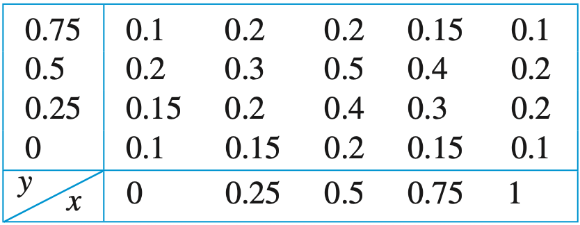
\(\Delta A = 0.25^2 = 0.0625\text{.}\) By the given data, the lower-left vertex sample points are:
\begin{align*} f(P_{11}) \amp= f(0, 0) \amp f(P_{12}) \amp= f(0, 0.25) \amp f(P_{13}) \amp= f(0, 0.50) \\ f(P_{21}) \amp= f(0.25, 0) \amp f(P_{22}) \amp= f(0.25, 0.25) \amp f(P_{23}) \amp= f(0.25, 0.50) \\ f(P_{31}) \amp= f(0.50, 0) \amp f(P_{32}) \amp= f(0.50, 0.25) \amp f(P_{33}) \amp= f(0.50, 0.50) \\ f(P_{41}) \amp= f(0.75, 0) \amp f(P_{42}) \amp= f(0.75, 0.25) \amp f(P_{43}) \amp= f(0.75, 0.50) \end{align*}
The Riemann sum \(S_{4,3}\) that corresponds to these lower-left vertex sample points is the following sum:
\begin{align*} S_{4,3} \amp= \sum_{i=1}^4 \sum_{j=1}^3 f(P_{ij}) \Delta A \\ \amp= 0.0625(0.1 + 0.15 + 0.2 + 0.15 + 0.2 + 0.3 + 0.2 + 0.4 + 0.5 + 0.15 + 0.3 + 0.4) \\ \amp\approx 0.190625 \end{align*}
Now by the given data, the upper-right vertex sample points are:
\begin{align*} f(P_{11}) \amp= f(0.25, 0.25) \amp f(P_{12}) \amp= f(0.25, 0.50) \amp f(P_{13}) \amp= f(0.25, 0.75) \\ f(P_{21}) \amp= f(0.50, 0.25) \amp f(P_{22}) \amp= f(0.50, 0.50) \amp f(P_{23}) \amp= f(0.50, 0.75) \\ f(P_{31}) \amp= f(0.75, 0.25) \amp f(P_{32}) \amp= f(0.75, 0.50) \amp f(P_{33}) \amp= f(0.75, 0.75) \\ f(P_{41}) \amp= f(1, 0.25) \amp f(P_{42}) \amp= f(1, 0.50) \amp f(P_{43}) \amp= f(1, 0.75) \end{align*}
The Riemann sum \(S'_{4,3}\) that corresponds to these upper-right vertex sample points is the following sum:
\begin{align*} S'_{4,3} \amp= \sum_{i=1}^4 \sum_{j=1}^3 f(P_{ij}) \Delta A \\ \amp= 0.0625(0.2 + 0.3 + 0.2 + 0.4 + 0.5 + 0.2 + 0.3 + 0.4 + 0.15 + 0.2 + 0.2 + 0.1) \\ \amp\approx 0.196875 \end{align*}
Taking the average of the two Riemann sums we have:
\begin{align*} \text{volume} \amp\approx \frac{S_{4,3} + S'_{4,3}}{2} = \frac{0.190625 + 0.196875}{2} = 0.19375 \end{align*}

15.1.17.

Use symmetry to evaluate the double integral
\begin{equation*} \iint_\c{R} \sin(x)\, dA\, , \qquad \c{R} = [0,2\pi] \times [0,2\pi] \end{equation*}
Solution.
We are asked to evaluate \(\ds \iint_\c{R} \sin(x)\, dA\) over the region \([0,2\pi] \times [0,2\pi]\) using symmetry.
Notice that the integrand \(f(x,y) = \sin(x)\) is completely independent of \(y\text{.}\) This means the solid is just the sine wave extended along the \(y\)-axis from \(y=0\) to \(y=2\pi\) (like a corrugated metal roof).
Let’s look at the cross-section of the surface along the \(x\)-axis. The function \(\sin(x)\) on the interval \([0, 2\pi]\) is perfectly symmetric about the \(x\)-axis. The "positive" volume above the \(xy\)-plane from \(x=0\) to \(\pi\) is exactly equal in magnitude to the "negative" volume below the \(xy\)-plane from \(x=\pi\) to \(2\pi\text{.}\)
Because these two identical volumes have opposite signs, they cancel each other out completely. Therefore:
\begin{equation*} \iint_\c{R} \sin(x)\, dA = 0 \end{equation*}

Exercise Group.

In the following exercises, evaluate the iterated integrals.
15.1.23.
\(\ds \int_{-1}^1 \int_0^\pi x^2\sin(y)\, dy \, dx\)
Solution.
We evaluate the inner integral first with respect to \(y\text{,}\) treating \(x\) as a constant:
\begin{align*} \int_0^\pi x^2\sin(y)\, dy \amp = x^2 \Big[ -\cos(y) \Big]_0^\pi \\ \amp = x^2 \big( -\cos(\pi) - (-\cos(0)) \big) \\ \amp = x^2 \big( -(-1) + 1 \big) = 2x^2 \end{align*}
Now, we substitute this back into the outer integral and integrate with respect to \(x\text{:}\)
\begin{align*} \int_{-1}^1 2x^2\, dx \amp = \left[ \frac{2}{3}x^3 \right]_{-1}^1 \\ \amp = \frac{2}{3}(1)^3 - \frac{2}{3}(-1)^3 \\ \amp = \frac{2}{3} + \frac{2}{3} = \frac{4}{3} \end{align*}
15.1.33.
\(\ds \int_0^4 \int_0^5 \frac{dy \, dx}{\sqrt{x + y}}\)
Solution.
We rewrite the integrand using a fractional exponent: \(\frac{1}{\sqrt{x+y}} = (x+y)^{-1/2}\text{.}\) Evaluating the inner integral with respect to \(y\) (treating \(x\) as a constant):
\begin{align*} \int_0^5 (x + y)^{-1/2}\, dy \amp = \left[ 2(x + y)^{1/2} \right]_{y=0}^{y=5} \\ \amp = 2(x + 5)^{1/2} - 2(x + 0)^{1/2} \\ \amp = 2\sqrt{x + 5} - 2\sqrt{x} \end{align*}
Now substitute this into the outer integral and integrate with respect to \(x\text{:}\)
\begin{align*} \int_0^4 \left( 2(x + 5)^{1/2} - 2x^{1/2} \right)\, dx \amp = \left[ 2\left(\frac{2}{3}\right)(x + 5)^{3/2} - 2\left(\frac{2}{3}\right)x^{3/2} \right]_0^4 \\ \amp = \frac{4}{3} \left[ (x + 5)^{3/2} - x^{3/2} \right]_0^4 \end{align*}
Evaluate at the boundaries:
\begin{align*} \amp \frac{4}{3} \Big( \big( (4+5)^{3/2} - 4^{3/2} \big) - \big( (0+5)^{3/2} - 0^{3/2} \big) \Big) \\ \amp = \frac{4}{3} \Big( (9^{3/2} - 4^{3/2}) - (5^{3/2} - 0) \Big) \\ \amp = \frac{4}{3} \Big( (27 - 8) - 5\sqrt{5} \Big) \\ \amp = \frac{4}{3} (19 - 5\sqrt{5}) \end{align*}

Exercise Group.

In the following exercises, evaluate the integral.
15.1.39.
\(\ds \iint_\c{R} \cos(x)\sin(2y)\, dA \, , \qquad \c{R} = \left[0,\frac{\pi}{2}\right] \times \left[0,\frac{\pi}{2}\right]\)
Solution.
We will evaluate this as an iterated integral. Let’s choose to integrate with respect to \(x\) first, treating \(y\) as a constant:
\begin{align*} \int_0^{\pi/2} \cos(x)\sin(2y)\, dx \amp = \sin(2y) \Big[ \sin(x) \Big]_{x=0}^{x=\pi/2} \\ \amp = \sin(2y) \left( \sin\left(\frac{\pi}{2}\right) - \sin(0) \right) \\ \amp = \sin(2y) (1 - 0) = \sin(2y) \end{align*}
Next, we substitute this result into the outer integral and integrate with respect to \(y\text{.}\) We’ll use a small u-substitution (\(u = 2y, du = 2dy\)):
\begin{align*} \int_0^{\pi/2} \sin(2y)\, dy \amp = \left[ -\frac{1}{2}\cos(2y) \right]_0^{\pi/2} \\ \amp = -\frac{1}{2}\cos\left(2\cdot\frac{\pi}{2}\right) - \left(-\frac{1}{2}\cos(0)\right) \\ \amp = -\frac{1}{2}\cos(\pi) + \frac{1}{2}\cos(0) \\ \amp = -\frac{1}{2}(-1) + \frac{1}{2}(1) = \frac{1}{2} + \frac{1}{2} = 1 \end{align*}
15.1.43.
\(\ds \iint_\c{R} x\ln(y)\, dA\, , \qquad \c{R} = [0,3] \times [1,e]\)
Solution.
We will set this up as an iterated integral. Let’s integrate with respect to \(x\) first, keeping \(y\) constant:
\begin{align*} \int_0^3 x\ln(y)\, dx \amp = \ln(y) \left[ \frac{1}{2}x^2 \right]_{x=0}^{x=3} \\ \amp = \ln(y) \left( \frac{1}{2}(3)^2 - \frac{1}{2}(0)^2 \right) \\ \amp = \frac{9}{2}\ln(y) \end{align*}
Now, we substitute this back into the outer integral and integrate with respect to \(y\text{.}\) Recall from MTH 252Z that integrating \(\ln(y)\) requires Integration by Parts (\(u = \ln(y), dv = dy\text{,}\) so \(du = \frac{1}{y}dy, v = y\)):
\begin{align*} \int_1^e \frac{9}{2}\ln(y)\, dy \amp = \frac{9}{2} \Big[ y\ln(y) - y \Big]_1^e \\ \amp = \frac{9}{2} \Big( \big( e\ln(e) - e \big) - \big( 1\ln(1) - 1 \big) \Big) \\ \amp = \frac{9}{2} \Big( (e(1) - e) - (0 - 1) \Big) \\ \amp = \frac{9}{2} \Big( 0 - (-1) \Big) = \frac{9}{2} \end{align*}

15.1.49.

  1. Which is easier, antidifferentiating \(\dfrac{y}{1 + xy}\) with respect to \(x\) or with respect to \(y\text{?}\) Explain.
  2. Evaluate \(\ds \iint_\c{R} \dfrac{y}{1 + xy}\, dA\text{,}\) where \(\c{R} = [0,1] \times [0,1]\text{.}\)
Solution.
  1. It is easier to antidifferentiate with respect to \(x\text{.}\) If we integrate with respect to \(x\text{,}\) the \(y\) in the numerator acts as a constant multiplier, and the expression looks like \(\int \frac{C}{1+Cx}\, dx\text{,}\) which yields a natural log function via a simple u-substitution.
    If we try to integrate with respect to \(y\) first, we have to deal with a \(y\) in both the numerator and denominator, which would require polynomial long division (or adding/subtracting a term) to simplify before integrating.
  2. Using Fubini’s Theorem, we will choose the easier path and integrate with respect to \(x\) first: \(dx\,dy\text{.}\)
    \begin{equation*} \int_0^1 \int_0^1 \frac{y}{1 + xy}\, dx\, dy \end{equation*}
    Inner integral with respect to \(x\text{:}\) let \(u = 1 + xy\text{,}\) then \(du = y\, dx\text{.}\)
    \begin{align*} \int_0^1 \frac{y}{1 + xy}\, dx \amp = \Big[ \ln|1 + xy| \Big]_{x=0}^{x=1} \\ \amp = \ln|1 + y| - \ln|1 + 0| = \ln(1 + y) \end{align*}
    Outer integral with respect to \(y\text{:}\)
    \begin{equation*} \int_0^1 \ln(1 + y)\, dy \end{equation*}
    We use Integration by Parts. Let \(u = \ln(1+y)\) and \(dv = dy\text{.}\) Then \(du = \frac{1}{1+y}dy\) and \(v = y\text{.}\) Alternatively, let \(w = 1+y\text{,}\) so \(dw = dy\text{,}\) and the bounds change from \([0,1]\) to \([1,2]\text{.}\) The integral becomes \(\int_1^2 \ln(w)\, dw\text{.}\) We know \(\int \ln(w)\, dw = w\ln(w) - w\text{.}\)
    \begin{align*} \int_1^2 \ln(w)\, dw \amp = \Big[ w\ln(w) - w \Big]_1^2 \\ \amp = (2\ln(2) - 2) - (1\ln(1) - 1) \\ \amp = 2\ln(2) - 2 - (0 - 1) \\ \amp = 2\ln(2) - 1 \end{align*}