Section14.2Limits and Continuity in Several Variables
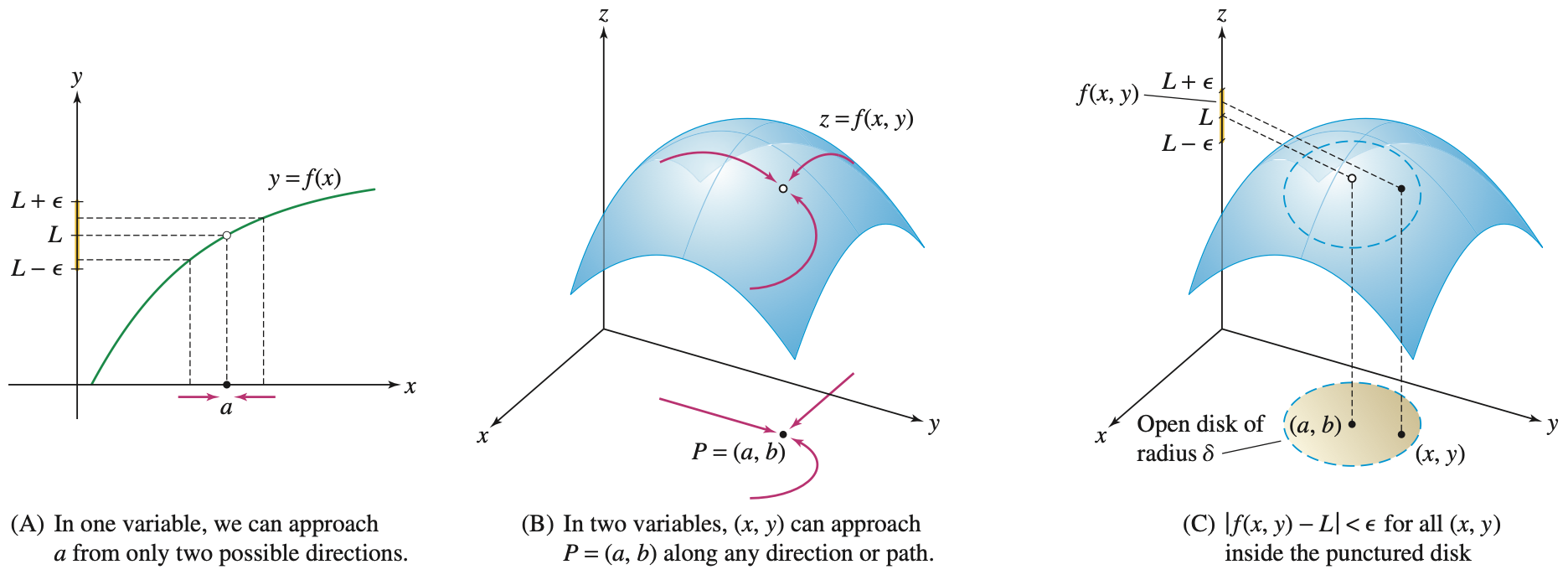
In our previous study of functions of a single variable, the concept of a limit was straightforward in one respect. We could only approach a point \(x=a\) from two directions, the left or the right. If the function approached the same value from both sides, the limit existed.
Now that we are working with functions of two variables, the domain is a plane. This means we can approach a point \((a,b)\) from infinitely many directions—along the \(x\)-axis, the \(y\)-axis, a diagonal line, a parabola, or even a spiral. This increase in freedom makes the definition of a limit more complex but also more interesting. In this section, we will learn how to determine if these limits exist and how to evaluate them.
Recall from MTH 251Z (or MH 251) that limits allow us to describe a function’s behavior near a specific point, even if the function is not defined at that point. The fundamental idea is that we can make the function’s output arbitrarily close to a limit value \(L\) by choosing inputs that are sufficiently close to the target point.
This is a calculus class, not a real analysis class, so we won’t be doing any epsilon-delta proofs in this class. Make sure you are comfortable with the limit idea informally. That is, the limit of a function at a point is the value that the function approaches as we get closer and closer to the point.
Recall back in MTH 251Z (or MTH 251), a function is continuous at a point if the limit of the function at that point is equal to the value of the function at that point. This is the same for functions of several variables.
That is, if we know that a function is continuous at a point (no hole, no jump, no asymptote), then we can evaluate the limit of the function at that point by directly substituting the point into the function.
Also recall back in MH 251Z (or MTH 251), a function is continuous at a point if the building blocks of the function are continuous at that point AND the function value is defined at that point.
Try arguing that the function \(f\) is continuous at \((-2,1)\text{.}\) Then you can evaluate the limit by directly substituting the point into the function.
Observe that \(z = 2x^2\) and \(z = 4x + y\) are both continuous at \((-2,1)\text{.}\) Also, the denominator \(4x + y\) is not equal to 0 at \((-2,1)\text{.}\) Hence, \(f\) is continuous at \((-2,1)\text{.}\)
Recall back in MTH 251Z (or MTH 251), the first step to evaluate a limit was to directly substitute the given point into the function. If things worked out, then great we found the limit! If not, then we had to do some some extra math to find the limit.
This is the same in limits of functions of several variables. If we can directly substitute the point into the function and get a number, then that number is (usually) the limit. If we don’t get a number (especially if we get an indeterminate form like \(\dfrac{0}{0}\)), then we have to do some extra work to find the limit.
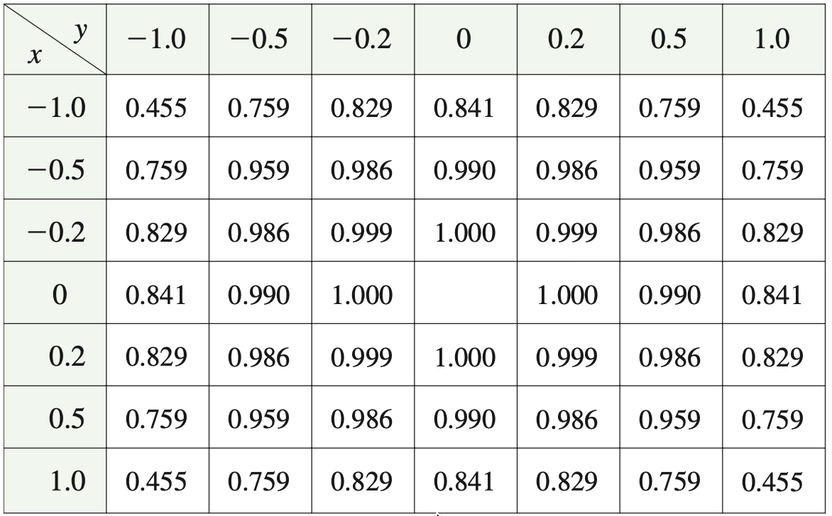
We can also try evaluating the limit using a table of values. Recall back in MTH 251Z (or MTH 251) that we want to see how the function behaves as we get closer and closer to the point \((0,0)\text{.}\) Then we can make a table of values for the function as BOTH \(x\) AND \(y\) approach 0.
Graphically, we can also see that the value of \(f(x,y)\) approaches 1 as we get closer to the point \((0,0)\) in any direction. This also suggests that
Unlike graphs of functions of a single variable where we can only approach a point from the left or the right, graphs of functions of several variables allow us to approach a point from infinitely many directions. To argue that a limit exists, we need to show that the function approaches the same value as we approach the point from any direction, like the previous example. If we can find two different directions that give different limit values, then the limit does not exist.
If you try direct substitution, you get \(\dfrac{0}{0}\text{,}\) which is an indeterminate form, which means we know nothing about the limits. Making a table of values or looking at graph can be helpful. Richard coded the graph below to help you visualize what the graph looks like.
Graphically, we can see that the value of \(f(x,y)\) approaches within a range of the \(z\) values between \(-1\) and \(1\text{...}\) We can’t determine a single value that the function approaches as we get closer to the point \((0,0)\text{.}\) Hence, the limit does not exist.
Without looking at the graph, we can also show that the limit does not exist by showing that the limit along different paths of approach give different values.
Observe that the limit along the line \(y = 0\) is 0, while the limit along the line \(y = x\) is \(\dfrac{1}{2}\text{.}\) Since we get different limit values along different paths of approach, the limit \(\ds \lim_{(x,y) \to (0,0)} \dfrac{xy}{x^2 + y^2}\) does not exist.
But how do we know if a limit exists without graphing the function? There are thousands of paths of approach to a point... How can we check all of them to see if they give the same limit value?
One way to improve our efficiency is to check the limit along a family of paths. For example, we can check the limit along ALL the linear paths by setting \(y = mx\) and seeing if the limit depends on the value of \(m\text{.}\) If so, then the limit does not exist.
This implies that the limit along the linear paths depends on the value of \(m\text{.}\) For example, if \(m = 0\text{,}\) then the limit is \(\dfrac{1 - 0^2}{1 + 0^2} = 1\text{.}\) If \(m = 1\text{,}\) then the limit is \(\dfrac{1 - 1^2}{1 + 1^2} = \dfrac{0}{2} = 0\text{.}\) Since we get different limit values along different paths of approach, the limit does not exist.
But... if we check the limit along the linear paths and get the same limit value, does that mean the limit exists? The short answer is no. There are other paths of approach than just the linear paths. If we find two different paths of approach that give different limit values, then the limit does not exist.
Observe that the limit along the path \(x = y^2\) is \(\dfrac{1}{2}\text{,}\) which is different from the limit along the linear paths. Since we get different limit values along different paths of approach, the limit does not exist.
One way to do so is to use some fancy calculus theorems to argue that there is only one possible limit value that the function can approach as we get closer to the point. One of such theorems is the Squeeze Theorem. In case you don’t recall what the Squeeze Theorem is from MTH 251Z (or MTH 251), below is a quick refresher.
A classic application of the Squeeze Theorem is to evaluate limits of functions involving some trigonometric functions like sine and cosine, since they are bounded between \(-1\) and \(1\text{.}\) So we can often convert the function to polar coordinates and try using the Squeeze Theorem to evaluate the limit.
Just a quick note that we don’t have to convert the function to polar coordinates to use the Squeeze Theorem if you can find some nice bounds for the function in terms of \(x\) and \(y\text{.}\) This usually happens when the function involves some trigonometric functions like sine and cosine, or other functions that are bounded between two numbers.
The problems listed below are assigned to be included in your problem set portfolio. Note that a specific selection of these problems will also form the written homework assignments. I recommend working through all of them to ensure a solid grasp of the material. Reach out to Richard for help if you get stuck or have any questions.
The solutions will be posted after the written homework due dates. If you have any questions about your work, talk to Richard and he is happy to discuss the process with you.
The function is the quotient of two continuous functions, and the denominator is not zero at the point \((1,1)\text{.}\) Therefore, the function is continuous at this point, and we may compute the limit by substitution.
This limit does not exist. Consider the following paths to the point \((x,y) = (0,0)\text{.}\) First along the line \(x = 0\) and second along the line \(y = x\text{.}\)
Let \(f(x,y) = \dfrac{x^3 + y^3}{xy^2}\text{.}\) Set \(y = mx\) and show that the resulting limit depends on \(m\text{,}\) and therefore the limit \(\ds \lim_{(x,y) \to (0,0)} f(x,y)\) does not exist.
So \(f\) is a constant along any line through the origin. Since \(\dfrac{m^3 + 1}{m^2}\) is not a constant function of \(m\text{,}\) the limit of \(f(x,mx)\) depends on \(m\text{.}\) For example,
The function \(\dfrac{1}{\sqrt{x^2 + y^2}}\) is continuous at the point \((3,4)\) since it is the quotient of two continuous functions and the denominator is not zero at \((3,4)\text{.}\) We compute the limit by substitution:
This limit does not exist. As \((x,y)\) approaches \((\pi,0)\text{,}\) the numerator approaches \(\cos\lp \pi \rp = -1\) and the denominator approaches \(\sin\lp 0 \rp = 0\text{.}\) This form \(-1/0\) indicates the limit will be unbounded. We can investigate the behavior by approaching along the line \(x = \pi\text{.}\)
We rewrite the function by dividing and multiplying it by the conjugate of \(\sqrt{x^2 + y^2 + 1} - 1\) and use the identity \((a - b)(a + b) = a^2 - b^2\text{.}\) This gives