In the previous section, we focused primarily on planes in \(\R^3\text{,}\) which has the form \(ax + by + cz = d\text{.}\) We will take a step further by exploring some curved surfaces in \(\R^3\) defined by second-degree polynomial equations.
In this section, we will introduce quadric surfaces, which are the three-dimensional analogs of conic sections studied in MTH 253 or MTH 253Z. This will give us a taste of the rich variety of surfaces and methods to analyze them in the second half of the class.
Quadric really just means "second degree". A quadric surface is a surface in \(\R^3\) that can be defined by a second-degree polynomial equation in three variables, typically denoted as \(x\text{,}\)\(y\text{,}\) and \(z\text{.}\) That is, the equation contains all the possible combinations of these variables up to the second degree.
There are 17 different types of quadric surfaces based on the CRC Standard Mathematical Tables. In this section, we will focus on the most common types in \(\R^3\text{.}\)
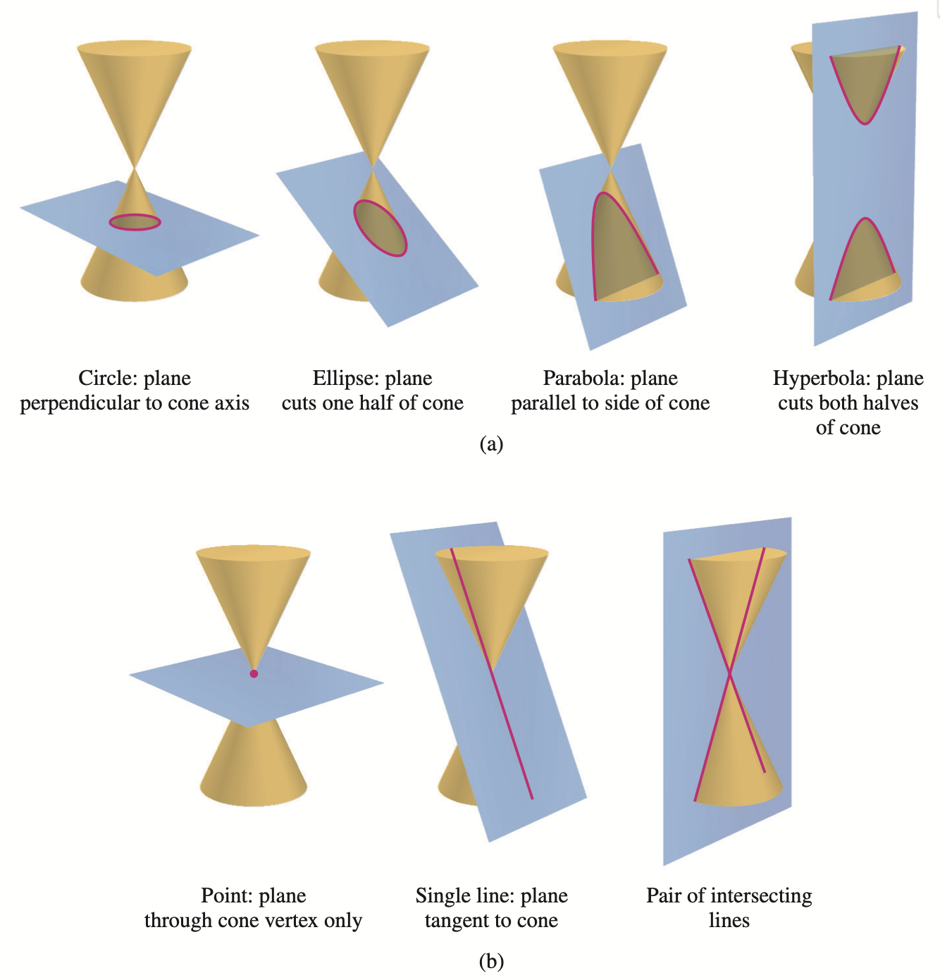
You may recall from MTH 253 or MTH 253Z a concept called the conic sections. These are the curves obtained by intersecting a plane with a double-napped cone. Depending on the angle and position of the intersecting plane, different types of conic sections can be formed, as shown in the following diagram.
The standard conic sections include circles, ellipses, parabolas, and hyperbolas. The degenerate conic sections include a point, a line, or two intersecting lines.
But why splitting the conic sections into these categories? This really comes down to the equations that define them. Recall that the equation of a conic section is really the general equation of a second-degree polynomial in \(\R^2\text{,}\) typically denoted as \(x\) and \(y\text{.}\)
\begin{equation*}
ax^2 + bxy + cy^2 + dx + ey + f = 0
\end{equation*}
where \(a, b, c, d, e, f\) are constants. The standard conic sections means the equation remains to be second-degree, while the degenerate conic sections means the equation reduces to first-degree or even a constant.
You may notice the similarity between the general equations of conic sections and quadric surfaces. In fact, quadric surfaces can be thought of as the three-dimensional analogs of conic sections. We add an additional variable \(z\) and consider second-degree polynomial equations in three variables instead of two.
Just like conic sections, quadric surfaces can also be classified into different types based on their equations and geometric properties. The goal of this section is to explore these different types of quadric surfaces, understand their equations, and visualize their shapes in \(\R^3\text{.}\)
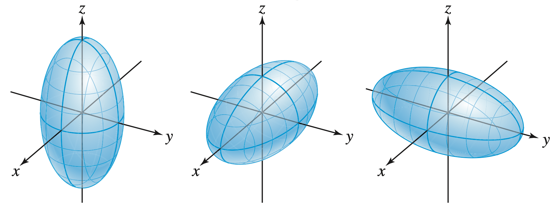
Observe that \(a\text{,}\)\(b\text{,}\) and \(c\) control the lengths of the semi-axes along the \(x\text{,}\)\(y\text{,}\) and \(z\) axes, respectively. When \(a = b = c\text{,}\) the ellipsoid becomes a sphere with radius \(a\text{.}\)
But how should we describe the ellipsoid in words? One way to do this is to use traces. Recall a trace is the curve obtained by intersecting a surface with a coordinate plane. Since a coordinate plane can be obtained by setting a variable to be a constant, the traces will be some curves in \(\R^2\text{.}\) So what the traces tell us is how the surface behaves when we "slice" it along the coordinate planes.
There are "standard" traces for quadric surfaces, which are obtained by setting one variable to be zero.
The \(xy\)-trace is obtained by setting \(z = 0\text{.}\) That is, we look at the curve obtained by intersecting the quadric surface with the \(xy\)-plane.
The \(xz\)-trace is obtained by setting \(y = 0\text{.}\) That is, we look at the curve obtained by intersecting the quadric surface with the \(xz\)-plane.
The \(yz\)-trace is obtained by setting \(x = 0\text{.}\) That is, we look at the curve obtained by intersecting the quadric surface with the \(yz\)-plane.
P.S.: Richard will use the "standard" traces here since they are the most easiest to work with (but not necessarily the most informative... but this is a good start! :D).
This is an ellipse on the \(xy\)-plane centered at the origin with semi-major axis length 3 along the \(y\)-axis and semi-minor axis length 2 along the \(x\)-axis.
This is an ellipse on the \(xz\)-plane centered at the origin with semi-major axis length 5 along the \(z\)-axis and semi-minor axis length 2 along the \(x\)-axis.
This is an ellipse on the \(yz\)-plane centered at the origin with semi-major axis length 5 along the \(z\)-axis and semi-minor axis length 3 along the \(y\)-axis.
We can imagine that the traces of the ellipsoid are all ellipses (or a point in the degenerate case) since slicing an ellipsoid with a plane will always yield an ellipse (or a point).
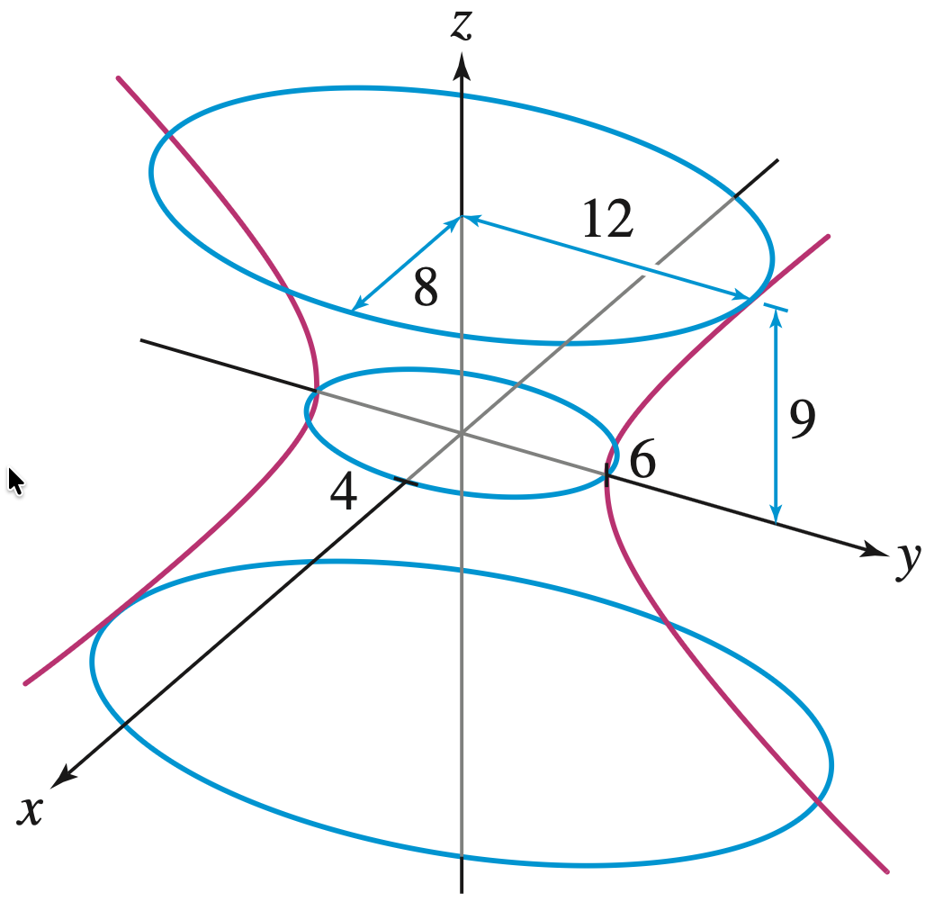
Observe that \(a\) and \(b\) control the lengths of the semi-axes along the \(x\) and \(y\) axes, respectively (so they control the size of the "waist"). But what about \(c\text{?}\)\(c\) is not shown directly on this hyperboloid...
One way to understand how \(c\) affects the shape of the hyperboloid is to look at its traces. Just like before, we will look at the "standard" traces obtained by setting one variable to be zero and see how the value of \(c\) affects them in the following example.
This is an ellipse on the \(xy\)-plane centered at the origin with semi-major axis length 5 along the \(x\)-axis and semi-minor axis length 3 along the \(y\)-axis.
This is a hyperbola on the \(xz\)-plane centered at the origin that opens along the \(x\)-axis. The vertices are located at \((\pm 5, 0)\text{,}\) and the asymptotes are given by the lines \(z = \pm \frac{7}{5} x\text{.}\)
This is a hyperbola on the \(yz\)-plane centered at the origin that opens along the \(y\)-axis. The vertices are located at \((0, \pm 3)\text{,}\) and the asymptotes are given by the lines \(z = \pm \frac{7}{3} y\text{.}\)
Observe that the value of \(c\) (in this problem, the \(7\)) affects the steepness of the hyperbolas in the \(xz\) and \(yz\) traces. A larger \(c\) value results in a steeper asymptotes in the traces, which means the hyperbolas are less "wide" compared to the waist; a smaller \(c\) value results in less steep asymptotes, which means the hyperbolas are more "wide" compared to the waist.
Observe that there is a gap between the two sheets of the hyperboloid. That is because the right-hand side of the equation \(\lp \frac{z}{c} \rp^2 - 1\) is negative when \(|z| \lt c\text{.}\) Yet the left side of the hyperboloid equation \(\lp \frac{x}{a} \rp^2 + \lp \frac{y}{b} \rp^2\) is always non-negative, so there are no points on the region when \(|z| \lt c\text{.}\)
Just like before, we can analyze the traces of the hyperboloid of two sheets to understand the surface. Feel free to try this as an exercise! Just one small hint here: there is no \(xy\)-trace since setting \(z = 0\) results in no points on the surface. If we set \(z = k\) for some \(|k| \gt c\text{,}\) we will get an ellipse as the trace instead.
The elliptic cone can be thought of as the transition surface between the hyperboloid of one sheet and the hyperboloid of two sheets.
If we increase the constant term on the right side of the elliptic cone by adding a \(1\text{,}\) the two(ish) sheets will move toward each other, creating a hyperboloid of one sheet.
If we decrease the constant term on the right side of the elliptic cone by subtracting a \(1\text{,}\) the two(ish) sheets will move away from each other, creating a hyperboloid of two sheets.
When the constant term on the right side of the hyperboloid equations is zero, we get the elliptic cone. Positive constant on the right-hand side means two sheets merge into one, while negative constant means one sheet splits into two.
Of course, we can analyze the traces of the elliptic cone as well. Try this as an exercise! If you play your cards right, you will find that the \(xy\)-trace is a point at the origin, while the \(xz\)- and \(yz\)-traces are pairs of lines through the origin. They are the three degenerate conic sections... Boring... But when you move up (or down) from the vertex along the \(z\)-axis, you will see that the traces are ellipses that grow larger as you move away from the vertex!
Similarly, the traces of the elliptic paraboloid can tell us a lot! Again, feel free to try this as an exercise. You will find that the \(xy\)-trace is a point at the origin, while the \(xz\)- and \(yz\)-traces are parabolas that open upward. Moving up along the \(z\)-axis from the vertex, you will see that the traces are ellipses that grow larger as you move away from the vertex!
The traces of the hyperbolic paraboloid are also very interesting! Try this as an exercise. You will find that the \(xy\)-trace is a point at the origin (aka the saddle point!), while the \(xz\)- and \(yz\)-traces are parabolas that open in opposite directions. Moving up along the \(z\)-axis from the saddle point, you will see that the \(xy\)-traces are hyperbolas that open along the \(y\)-axis, while moving down along the \(z\)-axis, the \(xy\)-traces are hyperbolas that open along the \(x\)-axis!
Now let’s take a pause and look back at what we have covered so far. We have learned six types of quadric surfaces. Make sure you know how to identify each type from its equation, and be able to analyze them using their traces (and sometimes the "standard" traces are not enough if we get the degenerate conic sections!).
To determine the type of quadric surface, we match the equation to the standard forms we have learned. Yet, there is no fractions on the \(x^2\) term and the \(z^2\) term... What to do?
Recall that we can always manipulate the equation algebraically to get it into a more recognizable form. For example, we know that \(2x\) can be rewritten as \(\lp \dfrac{x}{\frac{1}{2}} \rp\) if we want to get some fractions out of it.
One is to rewrite the equation into a more recognizable form, then use the standard sketch as a starting point. But the downside is that we may not be able to match it to a standard form easily, especially when there are some slight alternations involved (then not only you will need to recognize the type of surface, but also the alternation).
The other approach is to analyze the traces of the surface, then sketch it based on the traces. This approach is more general and works for any surface, but it may take more time and effort.
Alternatively, you can just put the equation into a 3D graphing tool (like GeoGebra or WolframAlpha) and get an instant sketch. But remember that Richard will not accept any calculator-generated answers without any justification on the exams.
The format matches the standard form of a hyperboloid of one sheet. Yet there is a slight alternation that \(y\) and \(z\) are swapped in their usual positions.
\(xy\)-trace: Setting \(z = 0\) gives \(4x^2 - y^2 = 9\text{.}\) This is a hyperbola opening along the \(x\)-axis, where the vertices are at \((\pm \dfrac{3}{2}, 0, 0)\) and the asymptotes are \(y = \pm \dfrac{2x}{3}\text{.}\)
\(xz\)-trace: Setting \(y = 0\) gives \(4x^2 + 9z^2 = 9\text{.}\) This is an ellipse centered at the origin with \(x\)-intercepts at \((\pm \dfrac{3}{2}, 0, 0)\) and \(z\)-intercepts at \((0, 0, \pm 1)\text{.}\)
\(yz\)-trace: Setting \(x = 0\) gives \(-y^2 + 9z^2 = 9\text{.}\) This is a hyperbola opening along the \(z\)-axis, where the vertices are at \((0, 0, \pm 1)\) and the asymptotes are \(z = \pm \dfrac{y}{3}\text{.}\)
In practice, it is often insanely difficult to sketch a surface from scratch, especially on paper. Richard is happy if you can describe the surface well either by matching things to the standard forms and point out any features (and also any alternation if any) or by analyzing the traces. This is a math class, not an art class!
We are still in the investigation of the standard quadric surfaces, but the following three types can be considered as special cases called quadratic cylinders. The term cylinder is used here in a more general sense, meaning that the surface extends infinitely in one direction (think about this as a vertical wall that goes up and down forever if the cylinder extends along the \(z\)-axis). They are a bit less interesting in the sense that their non-degenerate traces are just conic section.
The first type of the quadratic cylinder is right circular cylinder that we have seen in earlier section. Its general equation is
\begin{equation*}
x^2 + y^2 = r^2
\end{equation*}
where \(r\) is a positive constant representing the radius of the circular cross-sections. The only interesting traces of this surface are the traces \(z = k\text{,}\) which are circles of radius \(r\text{.}\)
where \(a\) and \(b\) are positive constants representing the semi-major and semi-minor axes of the elliptical trace. The interesting traces are again the traces \(z = k\text{,}\) which are ellipses with semi-major axis \(a\) and semi-minor axis \(b\text{.}\)
Again, the only interesting traces are the traces \(z = k\text{,}\) which are hyperbolas opening along the \(x\)-axis with vertices at \((\pm a, 0, k)\) and asymptotes \(y = \pm \dfrac{b}{a} x\text{.}\)
Last but not least, we have the parabolic cylinder, whose general equation is
\begin{equation*}
y = ax^2
\end{equation*}
where \(a\) is a nonzero constant that controls the "width" of the parabolic traces. The interesting traces are the traces \(z = k\text{,}\) which are parabolas opening along the \(y\)-axis with vertex at \((0, 0, k)\text{.}\)
Observe that all these quadratic cylinders can be obtained by extending a conic section (circle, ellipse, hyperbola, or parabola) along an axis perpendicular to the plane containing the conic section. That is, there is nothing interesting going on in the third dimension for these surfaces. Some people believe that the quadratic cylinders are essentially some degenerate cases of the quadric surfaces.
Your textbook include a summary page for this section (page 724). I recommend you organize your notes to include a similar summary page for your reference (with more details if you like). Again, Richard cares more about your understanding and the ability to analyze surfaces than sketching a perfect surface by hand!
The problems listed below are assigned to be included in your problem set portfolio. Note that a specific selection of these problems will also form the written homework assignments. I recommend working through all of them to ensure a solid grasp of the material. Reach out to Richard for help if you get stuck or have any questions.
The solutions will be posted after the written homework due dates. If you have any questions about your work, talk to Richard and he is happy to discuss the process with you.
In the following exercises, state whether the given equation defines an ellipsoid or hyperboloid, and if a hyperboloid, whether it is of one or two sheets.
The equation \(x^2 + \lp \frac{y}{4} \rp^2 + z^2 = 1\) defines an ellipsoid. The \(xz\)-trace is obtained by substituting \(y = 0\) in the equation of the ellipsoid. This gives the equation
The quadric surface is an ellipsoid, since its equation has the form \(\lp \frac{x}{a} \rp^2 + \lp \frac{y}{b} \rp^2 + \lp \frac{z}{c} \rp^2 = 1\) for \(a = 1\text{,}\)\(b = 4\text{,}\) and \(c = 1\text{.}\) To find the trace obtained by intersecting the ellipsoid with the plane \(z = \frac{1}{4}\text{,}\) we set \(z = \frac{1}{4}\) in the equation of the ellipsoid. This gives
The ellipsoid intersets the \(x\text{,}\)\(y\text{,}\) and \(z\) axes at the points \((\pm 4,0,0)\text{,}\)\((0,\pm 2, 0)\text{,}\) and \((0,0,\pm 2)\text{,}\) hence (B) is the corresponding figure.
The \(x\text{,}\)\(y\text{,}\) and \(z\) intercepts are \((\pm 2,0,0)\text{,}\)\((0,\pm 4, 0)\text{,}\) and \((0,0,\pm 2)\) respectively, hence (A) is the correct figure.
The \(x\text{,}\)\(y\text{,}\) and \(z\) intercepts are \((\pm 2,0,0)\text{,}\)\((0,\pm 2, 0)\text{,}\) and \((0,0,\pm 4)\) respectively, hence theh corresponding figure is (C).
The hyperboloid in the figure is of one sheet and the intersections with the planes \(z = z_0\) are ellipses. Hence, the equation of the hyperboloid has the form
By the given information this ellipse has \(x\) and \(y\) intercepts at the points \((\pm 2, 0, 0)\) and \((0, \pm 3, 0)\text{,}\) hence \(a = 4\) and \(b = 6\text{.}\)